Chapter 5 - Implementation and evaluation of SOM based recommendation techniques
SOM implementation
We implemented a basic SOM based on the (Original) Incremental SOM Algorithm as described by Kohonen in [kohonen01som] which has been rigorously introduced and described in the previous chapters.
We make use of a set of N sparse data vectors, all vectors have the same dimensionality but will not have values for all dimensions. During training the dimensions in which a data vector misses values will be ignored, in the distance calculation carried out when finding the BMN for a data vector missing values are assumed to contribute 0 to the distance and when updating the reference vector only the dimensions in which the data vector has values are updated.
Alternative methods for handling missing values were tested, such as using default values for missing values during the distance and/or updating. Positive results could be obtained with default values, however we are still unsure about the validity of using default values. It seems that sparsity of data and insertion of default values will result in e.g. the distance calculations being dominated by the default values, hence we chose to not use default values for our implementation in the end.
The SOM algorithm will form a projection of high dimensional data manifolds onto a regular array. The elements of the array are as previously mentioned referred to as nodes . The regular array has a rectangular lattice structure (nodes are arranged in rectangular patterns) and a sheet shape (nodes on the edges of the array do not "wrap around" to the "other side"). The nodes of the array are referred to using their index  where
where  is always the top left node and
  the bottom rightmost node. A Euclidean distance measure is used to determine distances between pairs of nodes in the array. We will henceforth refer more generally to the regular array as a "map". This terminology is appropriate both as the visualization of data on the grid looks like a map, and the SOM itself is a mapping defined by the regular array and the reference vectors associated with the elements of the array.
With each node a reference vector is associated and of the same dimensionality as the vectors in V . The number of rows and columns in a map M is accessed using the notation  and
and  respectively. The reference vector for a node in the map is retrieved using the index of the node, e.g. M0, 0 specifies the reference vector for the top-left node in the map. A element i ∈ M is an index tuple, e.g.
  for the top left node, which can also be used to specify a reference vector in the map using the notation Mi , in which case a specific dimension of the reference vector can be specified using the notation Mi(d) .
We initialize the reference vectors for each node in the array by picking random samples from the training vectors. While this is not an optimal initialization method, it seems to work well enough for us.
The training of a SOM requires specifying the parameters listed in [som parameters] the parameters include the size of the map and the settings for the rough order and fine tuning phase of training the SOM.
| Map | |
| rows | Number of rows in the array. |
| columns | Number of columns in the array. |
| Rough ordering phase | |
| RoughT | Number of training iterations. |
 |
Initial learning rate for training. |
 |
Initial neighborhood radius for training. |
 |
Final neighborhood radius for training. |
| Fine tuning phase | |
| FineT | Number of training iterations. |
 |
Initial learning rate for training. |
 |
Initial neighborhood radius for training. |
 |
Final neighborhood radius for training. |
som parameters
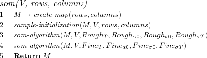
The function create-map on line 1 tells us that a map structure as previously described is created and consists of the specified number of rows and columns .
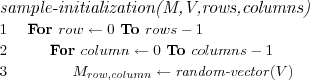
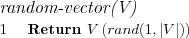
The sample-initialization method simply picks a random vector from the set V repeatedly using the random-vector method as shown. The random selection means that some data vectors might be used for multiple reference vectors as initialization, while this might seem problematic, i.e. how will a BMN be determined if multiple reference vectors are equally "close" to a sample during training, this is however not a problem as we will simply pick the first found BMN as closest and adjust it, no winner takes all situation will (or is likely to) arise as we also adjust the neighboring node's reference vectors, in the end the adjustments will even out.
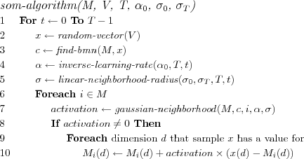
We chose to implement a stochastic SOM algorithm. Thus one random data (sample) vector at the time will be selected from the training data and shown to the SOM whereby the currently best matching node (BMN) for the sample is directly found, and the reference vector for the BMN, and the reference vectors for nodes in its neighborhood, are directly adjusted to become more similar to the sample. Since this is a incremental algorithm, time is equivalent to the current iteration number , starting from 0.
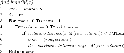
The BMN for a sample data vector is found by computing the Euclidean distance between the sample and each node's reference vector, the node which's reference vector is nearest the sample is chosen as BMN.
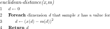
The euclidean distance calculation as already mentioned and motivated ignores dimensions in which the sample x has no values.
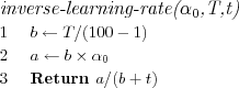
We used an inverse of time learning rate function which decreases inversely with time towards zero (but does not become zero, which would cause a division by zero error, it approaches roughly a hundredth of the initial learning rate).
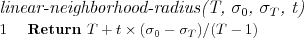
We used a linear neighborhood radius which decreases linearly from the initial neighborhood radius down to 1.
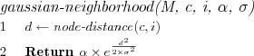
We use a gaussian function to implement the neighborhood function, i.e. a guassian neighborhood function . Neighboring nodes i within the radius σ at time t of the BMN c have a higher activation than nodes outside the radius σ . The learning rate α decides how much can at most be learned at any time t , i.e. the maximum activation.
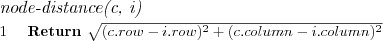
The distance between the BMN c and the neighboring node i is calculated using the node-distance function, which uses the row and column indices of the nodes to determine the distance between the node's index vectors on the regular array. Please note that this does not at all involve using the node's reference vectors, it only depends on the structure of the map.)
SOM based recommendation techniques
As in Part I recommendation techniques will be described using simple pseudo code that outlines how available profile models are used to generate recommendations.
For all the described techniques the common assumption is made that all the rating data uses the same rating scale ![[R_{min},R_{max}]](image/math160.png) . It is always assumed that there is a set
. It is always assumed that there is a set 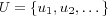 and
and  consisting of all users and items respectively for which necessary profile models are available. The profile models previously presented in Part I will again be used.
The techniques that generate predictions outline how to predict ratings on all available items for all available users on items the users have not rated, this gives a better idea of the complexity of the algorithm than simply showing how to predict for the active user on the active item. The techniques do not outline nor discuss how to introduce new users or items into the system.
The techniques in addition to assuming the presence of required profile models also assume that necessary constants have been specified.
SOM User based Collaborative Filtering (SOMUCF)
Recommendation technique based on the CF approach. Makes use of the neighborhood preservation of data in the SOM to retrieve similar users for the active user. The active user's neighborhood is simply all other users that have the same BMN as the active user, and users having neighboring nodes as BMN. The constant NR (Neighborhood Radius) specifies the radius within which neighboring nodes of the BMN can be found in the SOM's map. Otherwise the technique is the same as the UCF technique.
Assume that each user u ∈ U has a user rating model ur , and that each item i ∈ I has a item rating model ir . Let M represent a trained SOM that has been trained on a set of item rating models.
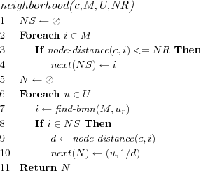
The function neighborhood(node, M, U, NR) determines which of the nodes in M lie within the neighborhood radius NR of the active user's BMN and returns the set of users in the neighborhood as well as their similarity with the active user.
In order to determine which nodes lie within the neighborhood radius NR of the BMN we use the node-distance function previously described. An alternative would have been to consider the distance between the node's model vectors. We did attempt this, however we didn't seem to get any better results doing this, probably because as our u-matrices indicate we don't have any clear clustering structure motivating its usage.
Finally the active user's neighbors are considered to be all the users u ∈ U in the BMN and its neighboring nodes. Neighbors having the same BMN as the active user are considered to be perfectly similar to the active user. Neighbors having a neighboring node as BMN are assigned a similarity based on their BMN's distance to the active user's BMN, we chose to implement this as a simple  formula, where d is the distance between the active user's BMN and the neighbor's BMN. Note that the shown neighborhood code is not optimal, only descriptive.
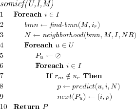
SOM Item based Collaborative Filtering (SOMICF)
The recommendation technique is based on the CF approach if the item SOM is based on rating data, however if it is based on attribute data it is based on the CBF approach. The technique is the same in both cases however, the difference lies in how the SOM is created which is beyond the scope of the technique.
Makes use of the neighborhood preservation of data in the SOM to retrieve similar items for the active item. The active item's neighborhood is simply all other items that have the same BMN as the active item, and items having neighboring nodes as BMN. The constant NR (Neighborhood Radius) specifies the radius within which neighboring nodes of the BMN can be found in the SOM's map. Otherwise the technique is the same as the ICF technique.
Assume that each user u ∈ U has a user rating model ur , and that each item i ∈ I has a item rating model ir . Let M represent a trained SOM that has been trained on a set of user rating models.
Item SOM User based Collaborative Filtering (ISOMUCF)
The recommendation technique is based on the CF approach if the item SOM is based on rating data, however if the item SOM is based on attribute data it is based on a hybrid filtering approach. The technique is the same in both cases however, the difference lies in how the SOM is created.
User similarities are calculated only over items similar to the active item. Prediction algorithm too is only provided with user rating models containing ratings on items similar to the active item, this means that for example user mean ratings will only be over items similar to the active item. It is conceivable that for certain types of movies the rating behavior of users varies, hence making it motivated to attempt to capture this when predicting. Makes use of the neighborhood preservation of data in the SOM to retrieve similar items for the active item. The active item's neighborhood is simply all other items that have the same BMN as the active item, and items having neighboring nodes as BMN. The constant NR (Neighborhood Radius) specifies the radius within which neighboring nodes of the BMN can be found in the SOM's map.
Assume that each user u ∈ U has a user rating model ur , and that each item i ∈ I has a item rating model ir . Let M represent a trained SOM that has been trained on a set of item rating models.
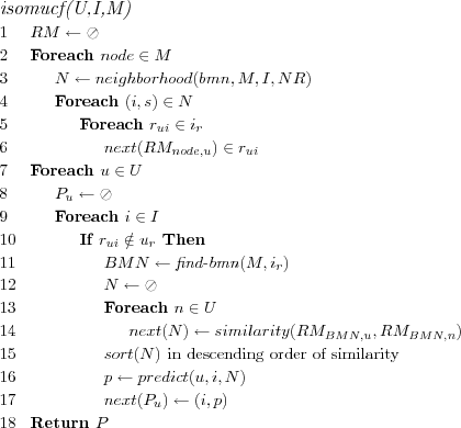
Line 6 creates the sets of ratings denoted RMnode, u , which are user rating sets consisting only of ratings on items within the neighborhood of the node in question. Thus during prediction we can given an active item's BMN easily retrieve rating models for users consisting only of ratings on items similar to the active item.
An alternative implementation of this technique is to completely skip the model building step on lines 1-6, which is time consuming and memory intensive. Instead having selected an active user and an active item, the active user's rating model is reduced to only contain ratings on items within the active item's neighborhood. This means that instead item neighborhoods should be modeled, which is less memory requiring. Neighbors models are not modified, instead similarity is computed directly with the active user's reduced rating model, which is in most cases such as with Pearson similarity exactly the same thing as had the neighbors model also been reduced. However, when predicting e.g. using Weighted Deviation From Mean, a difference will arise because we are still working with the neighbors complete rating models, their mean will not be over items similar to the active item but over all their items. We implemented and evaluated both these methods, however results appeared to be almost similar for both approaches, since the technique as it is presented here has a more theoretical sound motivation we choose to only present its results.
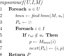
Model Predicting SOM User based Collaborative Filtering (MPSOMUCF)
Recommendation technique based on the CF approach. The value specified for each item by the model vector of the BMN for the active user is used as predictions for all items for the active user.
Assume that each user u ∈ U has a user rating model ur . Let M represent a trained SOM that has been trained on a set of user rating models.
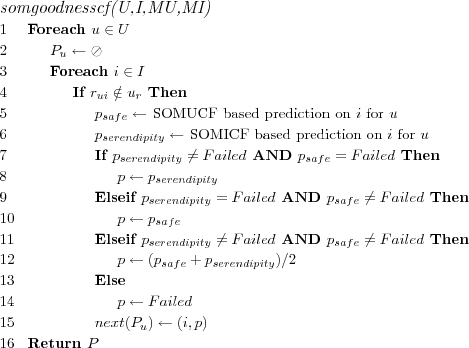
SOM Goodness Collaborative Filtering (SOMGOODNESSCF)
Recommendation technique combines the SOMUCF and SOMICF technique and uses the average of the two techniques predictions as a goodness prediction. Note that if the item SOM used by the SOMICF technique is based on attributes and not ratings, then this combined technique will be based on the HF approach. The SOMUCF based predictions are considered to have a possible element of serendipity, while the SOMICF based predictions to be more safe. By taking into account these two predictions a final goodness prediction can be made, the simplest choice of taking the average of the two prediction was made in this technique. Depending on whether
Assume that each user u ∈ U has a user rating model ur , and that each item i ∈ I has a item rating model ir . Let MU represent a trained SOM that has been trained on a set of user rating models, and let MI represent a trained SOM that has been trained on a set of item rating models.
Top-N SOM User based Collaborative Filtering (TOPNSOMUCF)
Recommendation technique makes predictions for users using the SOMUCF recommendation technique and creates Top-N ranking lists by sorting the predictions for each user in descending order of prediction and recommending the Top-N items with highest predictions.
Top-N SOM Item based Collaborative Filtering (TOPNSOMICF)
Recommendation technique makes predictions for users using the SOMICF recommendation technique and creates Top-N ranking lists by sorting the predictions for each user in descending order of prediction and recommending the Top-N items with highest predictions.
Top-N SOM Goodness Collaborative Filtering (TOPNSOMGOODNESSCF)
Recommendation technique makes predictions for users using the SOMGOODNESSCF/CBF recommendation technique and creates Top-N ranking lists by sorting the predictions for each user in descending order of prediction and recommending the Top-N items with highest predictions.
Evaluation data
The rating and attribute data sets presented previously in Part II were used again, this time split over users into a 80% training data set and a 20% test data set. The training data set was used to create a SOM, the user models in the training data set and the item models in the training set were respectively used to create a user SOM and a item SOM. Thus for i.e. the DS dataset the same 80% training set was used to create a item SOM as well as a user SOM, the idea being to use evaluation datasets created similarly to those used in Part I. However we must emphasize that we chose for simplicity (on behalf of reliability of validation results, which we however still consider representative of what can be obtained with the recommendation algorithms in question) to make simple Hold Out evaluations instead of K-Fold Cross Validations.
This time we decided to use the IMDb keyword lists, which provides for each movie a set of descriptive IMDb user specified keywords. The keyword lists were preprocessed to only contain keywords used for at least 5 different movies and at most for 50 different movies, it was also required that each movie had at least 5 keywords. See [soms] for further information about the SOM's generated based on the evaluation datasets.
| Map | Rough ordering | Fine tuning | SOM Evaluation | ||||||||||
| SOM | Rows | Columns | T | α | σ0 | σT | T | α | σ0 | σT | Runtime | AQE | TE |
| IMDBK | 50 | 50 | 1000 | 0.9 | 20 | 3 | 100000 | 0.2 | 3 | 1 | 16min | 1.653 | 0.470 |
| DS2-ITEM | 20 | 20 | 1000 | 0.9 | 20 | 3 | 200000 | 0.2 | 3 | 1 | 13min | 3.803 | 0.043 |
| DS2-USER | 20 | 20 | 1000 | 0.9 | 20 | 3 | 200000 | 0.2 | 3 | 1 | 13min | 3.981 | 0.054 |
| DS-ITEM | 20 | 20 | 1000 | 0.9 | 20 | 3 | 200000 | 0.2 | 3 | 1 | 5min | 2.033 | 0.307 |
| DS-USER | 20 | 20 | 1000 | 0.9 | 20 | 3 | 200000 | 0.2 | 3 | 1 | 16min | 4.556 | 0.047 |
| CML-ITEM | 20 | 20 | 1000 | 0.9 | 20 | 3 | 200000 | 0.2 | 3 | 1 | 16min | 3.903 | 0.075 |
| CML-USER | 20 | 20 | 1000 | 0.9 | 20 | 3 | 200000 | 0.2 | 3 | 1 | 21min | 5.792 | 0.002 |
soms
The DS2 dataset when used to create an item SOM has the advantage of containing few items that have been rated by only a few users, the DS dataset on the other hand contains some items that have been rated by very few users and because of this we're likely to see some kind of neighborhood formation based only on the fact the item's share the fact that few users have rated them.
The IMDBK dataset contains only 609 of the items in the CML dataset, the SOM is also very large, which must be taken into account when interpreting the evaluation results (especially the coverage).
Evaluation results
The recommendation techniques were evaluated for the evaluation datasets using various combinations of evaluation protocol and evaluation metrics.
For the recommendation techniques we select where necessary an appropriate combination of similarity and prediction algorithm, we use a decent set of settings giving good results, not necessarily the absolute best results, but near enough to be interesting to list.
We will describe briefly for each recommendation technique the setup of the evaluation, such that the evaluation can easily be understood and reproduced.
Accuracy of predictions
The result tables use the following abbreviations for the column headings: ET = Evaluation time (in minutes), Us = Usuccessful , Uf = Ufailed , Ps = Psuccessful , Pf = Pfailed , Cov = Coverage, Corr = Correctness.
For the settings name the name of the dataset from which prediction evaluation data was generated is always displayed first, i.e. DS, DS2 or CML. Usually the SOM that is needed by recommendation technique being evaluated is based on the same evaluation dataset. However the settings named CML-IMDBK use the IMDb keyword SOM, the prediction evaluation is still based on a evaluation dataset based on the CML dataset. Each table of evaluation results is followed by description of algorithms and settings used for each evaluation.
Where applicable the value of the neighborhood radius NR is indicated in the settings name, e.g. DS-NR3 means a neighborhood radius of 3 (NR=3) was used for that setting.
In all cases a Hold Out evaluation was performed using rating data split over users such that 80% of each users ratings are used for training data and 20% of each users ratings used as test data. Note that the same Hold Out evaluation data was used for each evaluation based on the same rating dataset, similarly the same SOM as previously described was used each time.
SOMUCF Technique
| Settings | ET | Us | Uf | Ps | Pf | Cov | Corr | MAE | MAER | MAEUA | MAERUA | NMAE | MSE | RMSE |
| DS-NR0 | 0 | 1578 | 423 | 9510 | 15683 | 37.7% | 42.4% | 0.769 | 0.743 | 0.775 | 0.749 | 0.192 | 1.062 | 1.030 |
| DS-NR3 | 0 | 1997 | 4 | 22679 | 2514 | 90.0% | 44.9% | 0.715 | 0.679 | 0.739 | 0.705 | 0.179 | 0.897 | 0.947 |
| DS2-NR0 | 0 | 1606 | 395 | 8996 | 12275 | 42.3% | 43.2% | 0.771 | 0.741 | 0.802 | 0.776 | 0.193 | 1.106 | 1.051 |
| DS2-NR3 | 0 | 1991 | 10 | 19949 | 1322 | 93.8% | 45.0% | 0.715 | 0.678 | 0.755 | 0.721 | 0.179 | 0.899 | 0.948 |
| CML-NR0 | 0 | 781 | 162 | 6860 | 12711 | 35.1% | 35.7% | 0.917 | 0.895 | 0.957 | 0.932 | 0.229 | 1.433 | 1.197 |
| CML-NR3 | 0 | 943 | 0 | 18323 | 1248 | 93.6% | 39.1% | 0.813 | 0.780 | 0.839 | 0.810 | 0.203 | 1.099 | 1.04 |
somucf
SOMICF Technique
| Settings | ET | Us | Uf | Ps | Pf | Cov | Corr | MAE | MAER | MAEUA | MAERUA | NMAE | MSE | RMSE |
| DS-NR0 | 0 | 1815 | 186 | 14829 | 10364 | 58.9% | 46.2% | 0.704 | 0.685 | 0.706 | 0.695 | 0.176 | 0.999 | 0.999 |
| DS-NR4 | 0 | 2001 | 0 | 24327 | 866 | 96.6% | 46.8% | 0.689 | 0.648 | 0.709 | 0.667 | 0.172 | 0.851 | 0.923 |
| DS2-NR0 | 0 | 1293 | 708 | 6464 | 14807 | 30.4% | 46.6% | 0.694 | 0.683 | 0.668 | 0.663 | 0.173 | 1.037 | 1.018 |
| DS2-NR4 | 0 | 1996 | 5 | 20654 | 617 | 97.1% | 47.1% | 0.695 | 0.656 | 0.728 | 0.697 | 0.174 | 0.894 | 0.945 |
| CML-NR0 | 0 | 807 | 136 | 8850 | 10721 | 45.2% | 38.9% | 0.840 | 0.835 | 0.865 | 0.866 | 0.210 | 1.334 | 1.155 |
| CML-NR4 | 0 | 943 | 0 | 19283 | 288 | 98.5% | 41.9% | 0.753 | 0.716 | 0.791 | 0.757 | 0.188 | 0.948 | 0.974 |
| CML-IMDBK | 1 | 544 | 399 | 2583 | 16988 | 13.2% | 34.5% | 0.954 | 0.950 | 0.978 | 0.979 | 0.239 | 1.671 | 1.292 |
| CML-IMDBK-NR4 | 1 | 876 | 67 | 10230 | 9341 | 52.3% | 34.7% | 0.912 | 0.889 | 0.980 | 0.964 | 0.228 | 1.400 | 1.183 |
| CML-IMDBK-NR8 | 1 | 924 | 19 | 12128 | 7443 | 62.0% | 35.7% | 0.862 | 0.834 | 0.927 | 0.906 | 0.216 | 1.209 | 1.100 |
somicf weighted sum
| Settings | NR | ET | Us | Uf | Ps | Pf | Cov | Corr | MAE | MAER | MAEUA | MAERUA | NMAE | MSE | RMSE |
| DS-NR4 | 4 | 0 | 2001 | 0 | 24327 | 866 | 96.6% | 46.0% | 0.696 | 0.657 | 0.715 | 0.679 | 0.174 | 0.859 | 0.927 |
| DS2-NR4 | 4 | 0 | 1996 | 5 | 20654 | 617 | 97.1% | 47.0% | 0.693 | 0.657 | 0.726 | 0.694 | 0.173 | 0.886 | 0.941 |
| CML-NR4 | 4 | 0 | 943 | 0 | 19283 | 288 | 98.5% | 42.3% | 0.748 | 0.709 | 0.785 | 0.749 | 0.187 | 0.934 | 0.966 |
| CML-IMDBK-NR4 | 4 | 1 | 876 | 67 | 10230 | 9341 | 52.3% | 34.7% | 0.903 | 0.885 | 0.972 | 0.961 | 0.226 | 1.376 | 1.173 |
| CML-IMDBK-NR8 | 8 | 1 | 924 | 19 | 12128 | 7443 | 62.0% | 36.1% | 0.855 | 0.825 | 0.915 | 0.884 | 0.214 | 1.188 | 1.090 |
somicf average rating
ISOMUCF Technique
| Settings | ET | Us | Uf | Ps | Pf | Cov | Corr | MAE | MAER | MAEUA | MAERUA | NMAE | MSE | RMSE |
| DS-NR0 | 2 | 975 | 1026 | 5540 | 19653 | 22.0% | 43.9% | 0.710 | 0.677 | 0.697 | 0.670 | 0.177 | 0.853 | 0.924 |
| DS-NR5 | 8 | 1984 | 17 | 22978 | 2215 | 91.2% | 47.8% | 0.673 | 0.633 | 0.700 | 0.662 | 0.168 | 0.810 | 0.900 |
| DS2-NR0 | 0 | 347 | 1654 | 1012 | 20259 | 4.8% | 45.0% | 0.729 | 0.682 | 0.671 | 0.607 | 0.182 | 0.901 | 0.949 |
| DS2-NR5 | 5 | 1934 | 67 | 18996 | 2275 | 89.3% | 47.6% | 0.677 | 0.635 | 0.715 | 0.681 | 0.169 | 0.822 | 0.907 |
| CML-NR0 | 0 | 530 | 413 | 2985 | 16586 | 15.3% | 37.4% | 0.834 | 0.814 | 0.836 | 0.823 | 0.208 | 1.145 | 1.070 |
| CML-NR5 | 2 | 943 | 0 | 18902 | 669 | 96.6% | 43.1% | 0.728 | 0.690 | 0.756 | 0.724 | 0.182 | 0.880 | 0.938 |
| CML-IMDBK | 1 | 276 | 667 | 690 | 18881 | 3.5% | 36.7% | 0.916 | 0.868 | 0.914 | 0.861 | 0.229 | 1.335 | 1.156 |
| CML-IMDBK-NR5 | 2 | 772 | 171 | 8860 | 10711 | 45.3% | 39.1% | 0.792 | 0.767 | 0.841 | 0.818 | 0.198 | 1.039 | 1.019 |
| CML-IMDBK-NR8 | 67 | 875 | 68 | 10889 | 8682 | 55.6% | 41.1% | 0.766 | 0.732 | 0.822 | 0.791 | 0.192 | 0.978 | 0.989 |
isomucf
MPSOMUCF Technique
| Settings | ET | Us | Uf | Ps | Pf | Cov | Corr | MAE | MAER | MAEUA | MAERUA | NMAE | MSE | RMSE |
| DS | 0 | 2001 | 0 | 24946 | 247 | 99.0% | 41.8% | 0.816 | 0.777 | 0.847 | 0.811 | 0.204 | 1.206 | 1.098 |
| DS2 | 0 | 2001 | 0 | 21271 | 0 | 100.0% | 43.9% | 0.758 | 0.718 | 0.803 | 0.765 | 0.190 | 1.029 | 1.014 |
| CML | 0 | 943 | 0 | 19545 | 26 | 99.9% | 38.3% | 0.814 | 0.784 | 0.837 | 0.806 | 0.203 | 1.085 | 1.041 |
mpsomucf
While the MAE is not always that much worse than the other MAEs obtained using the SOM based recommendation techniques it is consistently the highest, however the prediction time is basically instantaneous, and as long as no new items are introduced coverage is near perfect.
SOMGOODNESSCF Technique
| Settings | ET | Us | Uf | Ps | Pf | Cov | Corr | MAE | MAER | MAEUA | MAERUA | NMAE | MSE | RMSE |
| DS | 0 | 2001 | 0 | 24809 | 384 | 98.5% | 46.8% | 0.683 | 0.640 | 0.702 | 0.662 | 0.171 | 0.814 | 0.902 |
| DS2 | 0 | 1998 | 3 | 21175 | 96 | 99.5% | 47.1% | 0.679 | 0.639 | 0.713 | 0.676 | 0.170 | 0.812 | 0.901 |
| ML | 0 | 943 | 0 | 19492 | 79 | 99.6% | 42.2% | 0.750 | 0.709 | 0.779 | 0.739 | 0.187 | 0.925 | 0.962 |
| CML-IMDBK | 1 | 943 | 0 | 19197 | 374 | 98.1% | 38.9% | 0.802 | 0.771 | 0.823 | 0.794 | 0.200 | 1.050 | 1.02 |
somgoodnesscf
Relevance of Top-N ranking lists
The result tables use the following abbreviations for the column headings: ET = Evaluation time (min), Us = Usuccessful , Uf = Ufailed , TNs = TNsuccessful , TNf = TNfailed , TNa , Cov = Coverage, R = Recall, P = Precision, U = Utility, RAU = RecallAU , PAU = PrecisionAU , UAU = UtilityAU .
In all cases, unless otherwise noted, a 20% Hold Out set was used that contained items assumed to all be relevant for a user (ratings ignored as explained before in Part I), the ability of the technique to return those items in the Top-N list was evaluated. Note that the same 20% Hold Out datasets were used for each evaluation. Keep in mind that
Where applicable the value of the neighborhood radius NR is indicated in the settings name, e.g. DS-NR3 means a neighborhood radius of 3 ( NR = 3 ) was used for that setting.
In all cases a top N = 10 list was generated for each user.
TOPNSOMUCF Technique
| Settings | ET | Us | Uf | TNs | TNf | TNa | Cov | R | P | F1 | U | AFHP | RAU | PAU | F1AU | UAU |
| DS-NR3 | 23 | 2001 | 0 | 15 | 1986 | 10 | 0.7% | 0.1% | 0.1% | 0.001 | 0.001 | 6 | 0.1% | 0.1% | 0.001 | 0.001 |
| DS2-NR3 | 6 | 2001 | 0 | 42 | 1959 | 10 | 2.1% | 0.2% | 0.2% | 0.002 | 0.003 | 5 | 0.2% | 0.2% | 0.002 | 0.003 |
| CML-NR3 | 0 | 943 | 0 | 79 | 864 | 10 | 8.4% | 0.5% | 1.0% | 0.007 | 0.008 | 5 | 0.7% | 1.0% | 0.006 | 0.008 |
topnsomucf
TOPNSOMICF Technique
| Settings | ET | Us | Uf | TNs | TNf | TNa | Cov | R | P | F1 | U | AFHP | RAU | PAU | F1AU | UAU |
| DS-NR4 | 50 | 2001 | 0 | 8 | 1993 | 10 | 0.4% | 0.0% | 0.0% | 0.000 | 0.000 | 6 | 0.0% | 0.0% | 0.000 | 0.000 |
| DS2-NR4 | 3 | 2001 | 0 | 102 | 1899 | 10 | 5.1% | 0.6% | 0.6% | 0.006 | 0.006 | 5 | 0.5% | 0.6% | 0.004 | 0.006 |
| CML-NR4 | 0 | 943 | 0 | 156 | 787 | 10 | 16.5% | 1.0% | 2.1% | 0.014 | 0.016 | 5 | 1.0% | 2.1% | 0.011 | 0.016 |
| CMl-IMDBK-NR4 | 1 | 943 | 0 | 216 | 727 | 10 | 22.9% | 1.4% | 2.9% | 0.019 | 0.023 | 5 | 2.1% | 2.9% | 0.019 | 0.023 |
topnsomicf weighted sum
| Settings | ET | Us | Uf | TNs | TNf | TNa | Cov | R | P | F1 | U | AFHP | RAU | PAU | F1AU | UAU |
| DS-NR4 | 50 | 2001 | 0 | 8 | 1993 | 10 | 0.4% | 0.0% | 0.0% | 0.000 | 0.000 | 7 | 0.0% | 0.0% | 0.000 | 0.000 |
| DS2-NR4 | 3 | 2001 | 0 | 83 | 1918 | 10 | 4.1% | 0.4% | 0.5% | 0.005 | 0.005 | 5 | 0.4% | 0.5% | 0.003 | 0.004 |
| CML-NR4 | 0 | 943 | 0 | 154 | 789 | 10 | 16.3% | 1.0% | 2.1% | 0.014 | 0.017 | 5 | 1.0% | 2.1% | 0.011 | 0.016 |
| CML-IMDBK-NR4 | 1 | 943 | 0 | 212 | 731 | 10 | 22.5% | 1.4% | 2.9% | 0.019 | 0.022 | 5 | 2.1% | 2.9% | 0.020 | 0.023 |
topnsomicf average rating
TOPNSOMGOODNESSCF Technique
| Settings | ET | Us | Uf | TNs | TNf | TNa | Cov | R | P | F1 | U | AFHP | RAU | PAU | F1AU | UAU |
| DS | 71 | 2001 | 0 | 5 | 1996 | 10 | 0.2% | 0.0% | 0.0% | 0.000 | 0.000 | 5 | 0.0% | 0.0% | 0.000 | 0.000 |
| DS2 | 9 | 2001 | 0 | 48 | 1953 | 10 | 2.4% | 0.2% | 0.3% | 0.003 | 0.002 | 6 | 0.2% | 0.3% | 0.002 | 0.002 |
| CML | 1 | 943 | 0 | 45 | 898 | 10 | 4.8% | 0.3% | 0.6% | 0.004 | 0.004 | 6 | 0.3% | 0.6% | 0.003 | 0.004 |
| CML-IMDBK | 2 | 943 | 0 | 25 | 918 | 10 | 2.7% | 0.1% | 0.3% | 0.002 | 0.002 | 6 | 0.2% | 0.3% | 0.002 | 0.002 |
topnsomgoodnesscf
Conclusions
The SOM based techniques do not perform better [comparision common som recommendation techniques] than the recommendation techniques presented in Part I, however the results do not discourage their use. The ISOMUCF technique and the SOMGOODNESSCF technique performs closest to the recommendation algorithm instances of the classic UCF technique as it was evaluated in Part I (i.e. using Pearson for similarity and Weighted Deviation From Mean for prediction). Notable is that we achieve almost 100% coverage by only using ~8% of all nodes. For the ranking list evaluations, similar or even worse results as those in Part I are obtained.
| Common | SOM based | |||||||
| DATASET | BASELINESF | UCF | ICF | SOMUCF | SOMICF | ISOMUCF | MPSOMUCF | SOMGOODNESSCF |
| DS | 0.687 | 0.679 | 0.727 | 0.715 | 0.689 | 0.673 | 0.758 | 0.679 |
| DS2 | 0.667 | 0.657 | 0.707 | 0.715 | 0.693 | 0.677 | 0.816 | 0.683 |
| CML | 0.754 | 0.729 | 0.744 | 0.813 | 0.748 | 0.728 | 0.814 | 0.750 |
comparision common som recommendation techniques
Recommendation techniques can be judged by many different qualities, MAE prediction accuracy is just one quality. Other qualities include their theoretical soundness (meaning something that seems intuitively correct, such as not only looking at how many movies two users have rated in common, but also determining the types of movies they have in common). In Part I the TRUSTUCF recommendation technique is used, which is a more sound recommendation technique than UCF as it tries to determine if a similar user has lots of experience of the type of movie he is to predict for. Another quality to judge a recommendation technique by is to which degree the technique implements transparency. Which quality to emphasize when selecting a technique, depends on the situation it will be used in. Does the situation motivate the additional complexity? In Part III we will use the concept of transparency when we visualize our recommendations.