Chapter 2 - Implementation and evaluation of common recommendation techniques
Everybody got mixed feelings. About the function and form. Everybody got to deviate from the norm.
RUSH
Recommender systems help users find interesting items among a large set of items within a specific domain by using knowledge about user's preferences in the domain. We will be working in the movie domain, applying common recommendation techniques to large sets of movie data. Although what we describe is aimed at the movie domain, much of what we describe also applies to other domains.
The architecture of a recommender system can be divided into three distinct, but tightly coupled, modules:
Recommendation profiles
Recommendation techniques
Recommendation interfaces
We will in this part focus on implementing recommender techniques with the intention of measuring their accuracy in terms of accurate predictions and accurate Top-N ranking lists, thus focus will lie only on the recommendation profiles and recommendation techniques. The recommendation techniques are the algorithms that produces predictions or Top-N ranking lists.
By prediction we will mean a value signifying how much a user will like a specific item, the prediction is usually, but not necessarily, on the same scale as the underlying rating data used to make the prediction. And by Top-N ranking list is meant a list of the most relevant items for a user sorted in decreasing order of relevance.
We will be using two common approaches for the recommender techniques that we will implement and evaluate.
A recommendation approach solves the problem of what will motivate a recommendation. Two common approaches are collaborative filtering and content based filtering. The CF approach relies on the opinions of a large group of users, whereas the CBF approach relies on pure facts.
A number of common recommendation techniques, some of which have already been introduced in Part I, build on the CBF and CF approach will be discussed, implemented and evaluated. In particular evaluation will be made based on three datasets, one is a modified version of the well known MovieLens rating dataset commonly used in scientific papers of this nature, the other two datasets, a rating and a transaction dataset, are collected from a Swedish e-commerce site selling DVD movies.
Evaluation will be performed using common accuracy and relevance metrics, a thorough explanation of the evaluation procedure and evaluation data will be given.
Recommendation profiles
Fundamental entities of any recommender system are user profiles and item profiles . The profiles are a necessary part of the recommendation process. It is important to consider both the contents of the profiles as well as the internal representation of the profiles. The profiles must contain enough information for the system to be able to make accurate recommendations based on them. The shape and amount of information differs from which approach is taken. We divide the process of creating profiles into two steps; information analysis focuses on which information is needed and how to collect it; profile analysis focuses on how to represent the profiles such that they can be used by the system in the recommendation process. The goal of this module is to create profiles that capture the taste and needs of the users and that are most descriptive of items.
Information analysis
There are two ways for the system to collect knowledge about a user's item preferences. Users can either explicitly enter their preferences into the system, by rating items or by filling out e.g. a form in which preferences can be described. Or the system can study how the users interact with the system and implicitly acquire knowledge about user preferences, for example the user's purchase history can be used as a implicit indication of preferred items, or site access logs can be used to determine which product pages are viewed more often by the user [schafer01ecommerce] .
Some form of feedback from the user is also desirable as the system can then improve future recommendations.
Information that represents users preferences can either be ratings for items or content based, e.g. movie genres and directors. Items can be represented by ratings given by users or by its content, e.g. attribute such as genre and director. Items can also be represented using keywords extracted from textual descriptions of the items, if such are available.
Once required data has been identified and collected, the actual profile representation needs to be considered.
Profile representation
It is necessary to represent the profiles in such a way that they can be used efficiently by the recommendation techniques to producing recommendations. The representation of the profiles is usually referred to as a model. Two classical representations is the user-item matrix model, commonly used by recommender systems implementing the CF approach, and the vector space model, commonly used in systems implementing the CBF approach. Montaner presents in [montaner03taxonomy] several different representations for profiles that have been proposed and used in different approaches. We will however be using simple set models for all profiles. User profiles will be represented as rating models and transaction models , and item profiles will be represented as rating models , transaction models and attribute models .
User rating models
A user rating model consists of all items rated by the user. That is, if u is a user, then ur is the (for simplicity assumed) non-empty set of items the user has rated and rui is the rating given to item i by the user. The number of items rated by the user is denoted using |ur| .
User transaction models
A user transaction model consists of all items the user has purchased. That is, if u is a user then ut is the (for simplicity assumed) non-empty set of items the user has purchased. The number of items purchased by the user is denoted using |ut| .
Item rating models
A item rating model consists of all users that have rated the item. That is, if i is a item, then ir is the (for simplicity assumed) non-empty set of users that have rated the item and rui is the rating given by user u to item i . The number of users that have rated the item is denoted using |ir| .
Item transaction models
A item transaction model consists of all users that have purchased the item. That is, if i is a item then it is the (for simplicity assumed) non-empty set of users that have purchased the item. The number of users that have purchased the item is denoted using |it| .
Item attribute models
A item attribute model consists of all attribute of one type that a item has. E.g. movies have many different types of attributes, such as genres, directors, actors, release year, keywords etc. A item's genre attribute model thus consists of all the movies genres. That is, if i is an item, then igenre is the non-empty set of all genres associated with the item. The number of genres that the item has is denoted using |igenre| . The same notation applies to any attribute type.
Recommendation techniques
Recommendation techniques will be described using simple pseudo code that outlines how available profile models are used to generate recommendations.
For all the described techniques the common assumption is made that all the rating data uses the same rating scale ![[R_{min},R_{max}]](image/math22.png) . It is always assumed that there is a set
. It is always assumed that there is a set  and
and  consisting of all users and items respectively for which necessary profile models are available. In some cases it will also be assumed that there is a set
  of attribute types. The profile models previously presented will be used.
The techniques that generate predictions outline how to predict ratings on all available items for all available users on items the users have not rated, this gives a better idea of the complexity of the algorithm than simply showing how to predict for the active user on the active item. The techniques do not outline nor discuss how to introduce new users or items into the system.
The techniques in addition to assuming the presence of required profile models also assume that necessary constants have been specified.
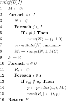
Baseline Statistical Filtering (BASELINESF)
Simple statistical recommendation technique for making predictions. The idea is to make use directly of the active user's rating model or the active item's rating model. Alternatively the whole populations opinion is used, however without forming any nearest neighborhoods or similar (collaborative filtering without neighborhoods). While rating data is assumed, it is not necessary for e.g. the random prediction algorithm, the ratings are then simply ignored, however the basic idea is that this baseline technique should serve as a statistical based baseline to compare other techniques against.
Assume that each user u ∈ U has a user rating model ur , and that each item i ∈ I has a item rating model ir .
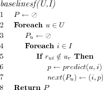
On line 7 the notation next(n) is introduced, this is a standard notation meaning that a new element is added to the next free index in the list N. It is necessary that N is a list as we wish to be able to sort the list and as the prediction algorithm will need to be able to iterate over it in sorted order.
User mean prediction algorithm
Uses the active user's rating mean as a prediction on all items for the active user.

Item mean prediction algorithm
Uses the active item's rating mean as a prediction for all users.

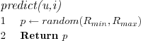
Random prediction algorithm
Makes a prediction by generating a uniformly random number in the rating interval. Multiple requests for a prediction on the same item for the same user may thus result in different predictions.
Population deviation from mean prediction algorithm
Considers the active user's mean rating and the entire populations deviation from their mean rating on the active item when making a baseline prediction.
User based Collaborative Filtering (UCF)
Recommendation technique based on the collaborative filtering approach. Predictions are based on a user neighborhood sorted in descending order of similarity with the active user. User similarities are calculated based on user rating models.
Assume that each user u ∈ U has a user rating model ur , and that each item i ∈ I has a item rating model ir .
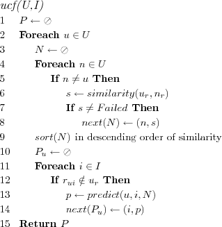
The neighborhood N created on lines 2-8 is the heart of the technique. The technique when creating the set of all neighbors for the active user u will only ignore neighbors for which no similarity can be calculated by the similarity algorithm. The idea is that it is up to a prediction algorithm to select a suitable subset of neighbors to use when predicting, but since the nearest neighborhood of users can be selected in many different ways the decision of how to do this is left upon a prediction algorithm.
In the evaluation we used this technique together with a similarity algorithm using the common Pearson correlation coefficient as a similarity measure and a prediction algorithm using the common weighted deviation from mean prediction function.
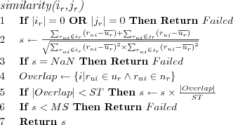
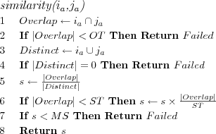
Pearson similarity algorithm
The Pearson correlation coefficient is used to determine similarity between two user (or item) rating models ur and nr .
The constants OT (Overlap Threshold or "Corated" Threshold), ST (Significance Weighting Threshold) and  (Minimum Negative/Positive Similarity Threshold) specify different threshold required for the similarity calculation to succeed. OT , MNS and MPS are not commonly used, but are shown here to demonstrate possible extensions to the similarity algorithm. ST is however commonly used and is recommended to be set between 20 to 50 [Herlocker, 00].
Similarity returned is a continuous value in the range [-1, +1] representing the similarity between two rating models. -1 means perfect dissimilarity. 0 means no linear correlation existed (note that if correlation can't be calculated or thresholds aren't met, Failed is returned, not 0), it is still possible the two rating models are dissimilar or similar. +1 means perfect similarity.
![\FUNCTION{similarity({$u_r$},{$n_r$})}
\LINE $Overlap \leftarrow \{i | r_{ui} \in u_r \wedge r_{ni} \in n_r\}$
\LINE If $|Overlap| < 2$ Then Return $Failed$
\LINE If $|Overlap| < OT$ Then Return $Failed$
\LINE \[s \leftarrow
\frac
{
\sum_{i \in Overlap}\left( r_{ui} \times r_{ni} \right) -
\frac
{\sum_{i \in Overlap} r_{ui} \times \sum_{i \in Overlap} r_{ni}}
{|Overlap|}
}
{\sqrt{
\left(
\sum_{i \in Overlap} r_{ui}^2 -
\frac
{\left( \sum_{i \in Overlap} r_{ui} \right)^2}
{|Overlap|}
\right)
\times
\left(
\sum_{i \in Overlap} r_{ni}^2 -
\frac
{\left( \sum_{i \in Overlap} r_{ni} \right)^2}
{|Overlap|}
\right)
}}\]
\LINE If $s = NaN$ Then Return $Failed$
\LINE If $|Overlap| < ST$ Then $s \leftarrow s \times \frac{|Overlap|}{s}$
\LINE If $MNS < s$ AND $s < MPS$ Then Return $Failed$
\LINE Return $s$](image/pseudo6.png)
The formula for calculating the Pearson correlation coefficient on line 4 uses no rating means and as such is suitable to use in any implementation of the formula as no separate mean calculation step for co-rated items is needed, the whole correlation coefficient can be calculated in one iteration over the set of co-rated items for the two users.
On line 5 there is a check whether the Pearson correlation coefficient is NaN, this check is needed as the denominator will sometimes be zero (occurs in extreme cases, such as when both users have rated 100 items, all with 5's).
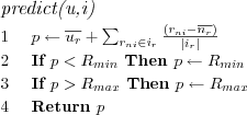
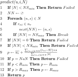
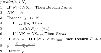
Weighted deviation from mean prediction algorithm
Neighbors weighted deviation from their mean rating is used when making a prediction. The constants NSmin (Minimum Neighborhood Size) and NSmax (Maximum Neighborhood Size) specify different thresholds required for the prediction to succeed. Note that the entire neighborhood is searched through for neighbors that have rated the active item, the algorithm does not simply consider e.g. the first NSmax neighbors when creating the neighborhood of predictors, this means that if the neighborhood is large enough then NSmax neighbors can usually be found, however they are most likely not always the neighbors with the highest similarity with the active user.
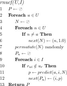
Random Neighbors User based Collaborative Filtering (RNUCF)
Recommendation technique based on the collaborative filtering approach. Predictions are based on a user neighborhood sorted in random order. No user similarities are calculated, instead all neighbors are assigned similarity 1.0 with the active user. The technique was only implemented in order to evaluate how the prediction algorithms used for the UCF technique work on a randomly sorted neighborhood. While we could have simply implemented prediction algorithms that creates a random nearest neighborhood, we chose to simply implement a second technique for the purpose. Assume that each user u ∈ U has a user rating model ur , and that each item i ∈ I has a item rating model ir .
Trust User based Collaborative Filtering (TRUSTUCF)
Recommendation technique based on the collaborative filtering approach. Predictions are based on a user neighborhood sorted in descending order of trust. Trust in a neighbor is a combination of the neighbor's similarity with the active user and the neighbors trusted ability to predict for the active item. User similarities are calculated based on user rating models. Users that have rated many of the items that are most similar to the active item are trusted to be able to predict reliably for it. Item similarities are calculated based on item rating models.
The constant MS (Model Size) specifies the size of the item neighborhoods to keep in memory. When trust is calculated for a neighbor, the trust will be based on how many of the MS most similar items to the active item the neighbor has rated.
Assume that each user u ∈ U has a user rating model ur , and that each item i ∈ I has a item rating model ir .
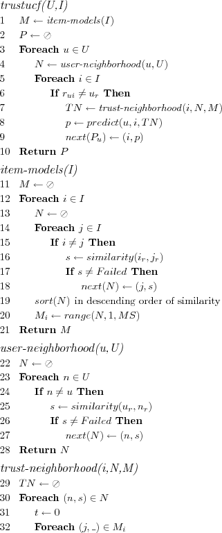
As can be seen on line 1 a model step is introduced in which item similarities for all items are precalculated, the MS most similar items for each item are saved. This step is necessary as it would be too costly to recalculate them each time they are needed. Note that on line 20 the range(L, S, E) method is introduced, this method simply extracts the elements on index S to E in the list L , additionally is  the whole list is returned.
On line 4 a regular user neighborhood N is calculated as in e.g. the UCF technique, for clarity it has been placed in a separate method. However unlike the UCF technique, the neighborhood will not be passed directly to the prediction algorithm. Instead, once an active item has been selected the neighborhood will on line 7 be passed to a method that modifies the neighbor similarities based on how much each neighbor is trusted to be able to predict for the active item. A neighbor that e.g. has not rated any item similar to the active is not trusted to be able to predict for the item at all and will have the similarity down weighted to zero.
Common Items Prioritizing User based Collaborative Filtering (CIPUCF)
Recommendation technique based on the collaborative filtering approach. Predictions are based on a user neighborhood sorted in descending order of common items with the active user. User similarities are still calculated with the active user, however the neighborhood is unlike the UCF technique not sorted based on the similarities. User similarities are calculated based on user rating models.
Assume that each user u ∈ U has a user rating model ur , and that each item i ∈ I has a item rating model ir .
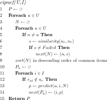
Line 9 will keep the previously calculated similarity between each neighbor and the active user, but the members of list N will be sorted according to the number of items they have in common with the active user (the step is thus quite simplified).
Item based Collaborative Filtering (ICF)
Recommendation technique based on the collaborative filtering approach. Predictions are based on a item neighborhood sorted in descending order of similarity with the active item. Item similarities are calculated based on item rating models.
The constant MS (Model Size) specifies the size of the item neighborhoods to keep in memory. The basic assumption is that item similarities, unlike user similarities in the UCF technique, are not likely to change as often/much as user similarities, hence a model can be build of item similarities.
Assume that each user u ∈ U has a user rating model ur , and that each item i ∈ I has a item rating model ir .
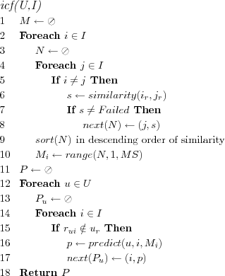
Keep in mind that the model size MS of the item similarity models Mi should be kept relatively small, If we assume that the majority of users have rated very few items, suppose around 20. If a excessively large item model size is then used, the prediction algorithm might (assuming it scans the entire item neighborhood for items the active user has rated) end up basing all predictions on the active users ratings on the same 20 items, simply because those 20 items are included in every single item's neighborhood. While those 20 items will have varying similarity with the active item, it is still important to keep this fact in mind, especially if the prediction algorithm ignores the item similarities (e.g. the Average Rating prediction algorithm).
Adjusted cosine similarity algorithm
The cosine angle is used as a similarity measure between two item rating models ir and jr , the cosine formula is applied to users deviations from their rating means instead of to their actual ratings. While this algorithm is expressed in terms of item rating models it works for user rating models as well, however [Sarwar et al., 01] considers the adjusted cosine formula more suitable for item rating models and suggests using Pearson for user rating models.
The constants OT (Overlap Threshold), ST (Significance Weighting Threshold) and MS (Minimum Similarity Threshold) specify different threshold required for the similarity calculation to succeed. OT and MS are not commonly used, but are shown here to demonstrate possible extensions to the similarity algorithm. ST is however just as applicable here as for the Pearson similarity algorithm.
Similarity returned is a continuous value in the range [-1, +1] representing the similarity between the two item rating models. Interpretation of similarities is similar to that of the Pearson similarity algorithm, -1 means perfect dissimilarity, +1 perfect similarity and 0 that nothing certain could be said about either case.
Average rating prediction algorithm
Calculates the active user's average rating on items that are similar to the active item. The average is used as a prediction. Unlike the baseline prediction algorithm that uses the active user's mean rating, this prediction algorithm uses a subset of the items the user has rated. The subsets consists of the items the active user has rated that are most similar to the active item.
The constants NSmin (Minimum Neighborhood Size) and NSmax (Maximum Neighborhood Size) specify different thresholds required for the prediction calculation to succeed.
Predictions are in the range ![[R_{min},R_{max}]](image/math28.png) .
.
Weighted sum prediction algorithm
Uses the active user's ratings on items that are most similar to the active item when making a prediction. The active user's ratings on items are weighted using the items similarity with the active item.
The constants NSmin (Minimum Neighborhood Size) and NSmax (Maximum Neighborhood Size) specify different thresholds required for the prediction calculation to succeed.
Predictions are in the range ![[R_{min},R_{max}]](image/math29.png) .
.
Random Neighbors Item based Collaborative Filtering (RNICF)
Recommendation technique based on the content based filtering approach. Predictions are based on a item neighborhood for the active item sorted in random order. No item similarities are calculated.
The constant MS (Model Size) specifies the size of the item neighborhoods to keep in memory.
Assume that each user u ∈ U has a user rating model ur , and that each item i ∈ I has a item rating model ir .
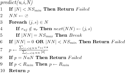
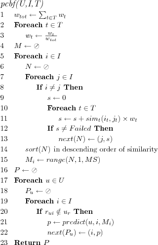
Personalized Content Based Filtering (PCBF)
Recommendation technique based on the content based approach. Predictions are based on a item neighborhood sorted in descending order of similarity with the active item. Item similarities are calculated based on item attributes. An item has one or more attribute type models, the total item similarity is a normalized weighted linear sum over all attribute models.
The ICF and PCBF techniques are similar, essentially only differing in how item similarities are calculated, however the fact the PCBF technique doesn't require any ratings on all items it predicts for (it is enough that the active user has rated some of the items similar to the active item) means a possibly increased coverage as long as attribute models are available for all items.
The constant MS (Model Size) specifies the size of the item neighborhoods to keep in memory.
Assume that each user u ∈ U has a user rating model ur , and that each item i ∈ I has a item rating model ir . Assume that each item has for each attribute type t ∈ T a attribute type model it. Assume that for each attribute type t there is a weight wt and a similarity measure simt .
Common attribute similarity algorithm
Defines similarity between two item attribute models as the ratio of shared attributes, against the total number of distinct attributes, between the two item attribute models.
The constants OT (Overlap Threshold), ST (Significance Weighting Threshold) and MS (Minimum Similarity Threshold) specify different threshold required for the similarity calculation to succeed. OT and MS are not commonly used, but are shown here to demonstrate possible extensions to the similarity algorithm.
Similarity returned is a continuous value in the range [0, 1] . 0 means no similarity and 1 means perfect similarity.
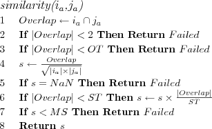
Cosine similarity algorithm
The cosine angle is used as a similarity measure between two item attribute models. Since attribute models are used the original cosine formula can be simplified significantly (as shown on line 4).
The constants OT (Overlap Threshold), ST (Significance Weighting Threshold) and MS (Minimum Similarity Threshold) specify different threshold required for the similarity calculation to succeed. OT and MS are not commonly used, but are shown here to demonstrate possible extensions to the similarity algorithm.
Similarity returned is a continuous value in the range [0, 1] . 0 means no similarity and 1 means perfect similarity.
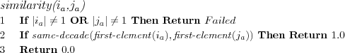
Same decade similarity algorithm
Assumes two item attribute models contain as first and only element a integer representing a year, the two attribute models are considered similar if they belong to the same decade. Since this is the movie domain, such a similarity measure makes sense, movies belonging to different decades can very roughly be seen to often have different characteristics.
Similarity returned is 1 if the two item attribute models belong to the same decade (in the same year) or 0 if they're from different decades.
Top-N User based Collaborative Filtering (TOPNUCF)
Recommendation technique makes predictions for users using the UCF recommendation technique and creates Top-N ranking lists by sorting the predictions for each user in descending order of prediction and recommending the Top-N items with highest predictions.
Top-N Item based Collaborative Filtering (TOPNICF)
Recommendation technique makes predictions for users using the ICF recommendation technique and creates Top-N ranking lists by sorting the predictions for each user in descending order of prediction and recommending the Top-N items with highest predictions.
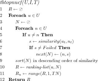
Top-N Personalized Content Based Filtering (TOPNPCBF)
Recommendation technique makes predictions for users using the PCBF recommendation technique and creates Top-N ranking lists by sorting the predictions for each user in descending order of prediction and recommending the Top-N items with highest predictions.
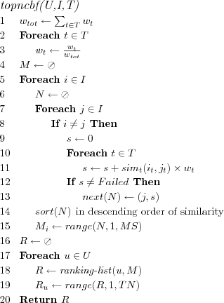
Top-N Content Based Filtering (TOPNCBF)
Recommendation technique makes Top-N ranking list recommendations based on item similarities. Item similarities are calculated based on attribute models.
The constant MS (Model Size) specifies the size of the item neighborhoods to keep in memory. The constant TN specifies the size of the Top-N ranking lists to recommend.
Assume that each user u ∈ U has a user rating model ur , and that each item i ∈ I has a transaction model it. Assume that each item has for each attribute type t ∈ T a attribute type model it. Assume that for each attribute type t there is a weight wt and a similarity measure simt .
Similar items ranking list algorithm
Ranking list is generated by considering items with all items purchased by the active user.
![\FUNCTION{ranking-list(u,M)}
\LINE $R \leftarrow \oslash$
\LINE Foreach $i \in u_t$
\LINE \INDENT Foreach $(i,s) \in M_i$
\LINE \INDENT \INDENT If $R[i] = NULL$ Then
\LINE \INDENT \INDENT \INDENT $R[i] = s$
\LINE \INDENT \INDENT Else
\LINE \INDENT \INDENT \INDENT $R[i] += s$
\LINE $sort(R)$ \COMMENT{in descending order of similarity}
\LINE Return $R$](image/pseudo21.png)
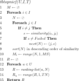
Transaction based Top-N User based Collaborative Filtering (TBTOPNUCF)
Recommendation technique makes Top-N ranking list recommendations based on a user neighborhood sorted in descending order of similarity with the active user. User similarities are calculated based on user transaction models.
The constant TN specifies the size of the Top-N ranking lists to recommend.
Assume that each user u ∈ U has a user rating model ur , and that each item i ∈ I has a transaction model it. Assume that each item has for each attribute type t ∈ T a attribute type model it. Assume that for each attribute type t there is a weight wt and a similarity measure simt .
Cosine similarity algorithm (Simplified transaction case)
The cosine angle is used as a similarity measure between two transaction models. The similarity algorithm is the same as for attribute models, except it works with transaction models.
Frequent items ranking list algorithm
Ranking list is generated by considering item frequencies among neighbors of the active user.
The constant NS (Neighborhood Size) specifies the (exact) number of neighbors of the active user to consider.
![\FUNCTION{ranking-list(u,N)}
\LINE If $|N| < NS$ Then Return $Failed$
\LINE $NN \leftarrow range(N,1,NS)$
\LINE $R \leftarrow \oslash$
\LINE Foreach $n \in NN$
\LINE \INDENT Foreach $i \in n_t$
\LINE \INDENT \INDENT If $R[i] = NULL$ Then $R[i] = 1$
%\LINE \INDENT \INDENT \INDENT $R[i] = 1$
\LINE \INDENT \INDENT Else $R[i]++$
%\LINE \INDENT \INDENT \INDENT $R[i]++$
\LINE $sort(R)$ \COMMENT{in descending order of similarity}
\LINE Return $R$](image/pseudo23.png)
Transaction based Top-N Item based Collaborative Filtering (TBTOPNICF)
Recommendation technique makes Top-N ranking list recommendations based on a item neighborhood sorted in descending order of similarity with the active item. Item similarities are calculated based on item transaction models.
The constant MS (Model Size) specifies the size of the item neighborhoods to keep in memory. The constant TN specifies the size of the Top-N ranking lists to recommend.
Assume that each user u ∈ U has a user rating model ur , and that each item i ∈ I has a transaction model it. Assume that each item has for each attribute type t ∈ T a attribute type model it. Assume that for each attribute type t there is a weight wt and a similarity measure simt .
Evaluation of recommender systems
Much theorizing has gone into optimum cell size. I think that history shows that a cell of three is best - more than three can't agree on when to have dinner
Professor Bernardo de La Paz
Recommender systems work with datasets to produce recommendations. Recommender systems that produce personalized recommendations always work with user datasets, such a dataset in current research consists of either user ratings or user "transactions" (information about which items a user has considered relevant). Evaluations are made of such recommender systems using all or parts of available user data as evaluation data, which is split into training and test data, and any of an assortment of suitable evaluation metrics.
An evaluation metric for a recommender system is currently focused either on accuracy of predictions, or relevance of Top-N ranking lists made by the recommender system [herlocker00understanding] .
In either case two simplifying assumptions are made, upon which all evaluations of the recommender system are based:
Given any training and test data, if the recommender system is able to accurately predict, based on the training data, ratings for items in the test data, then we assume the recommender system will also predict correctly for new unknown data.
Given any training and test dataset, if the Top-N list generated by the recommender system contains items from the test data, then the Top-N list is better than a Top-N list not containing any items from the test data.
Both of these assumptions are flawed, if the recommender system predicts badly for the test data it may still predict perfectly for future data. And if a Top-N list contains no relevant items, it may still be the case all items are relevant.
The user data available is not complete, and typically can not be complete. Hence no evaluation metric can give a true measure of how accurate the recommender system is on all future data. The evaluation metrics however give a true measure of how accurate the recommender system is on a specific evaluation dataset. Whether or not this accuracy holds for any future data is not guaranteed, and is not measured either.
In order to reliably evaluate an recommender system on a given evaluation dataset, a sensible and motivated choice of forming training and test datasets is highly necessary as well as a reliable evaluation protocol.
If evaluation results are to be compared against other evaluation results, it is necessary to make sure the evaluation datasets and evaluation protocols used for both evaluations are similar (preferably identical), otherwise comparisons and claims of better or worse results should not be made or at the very least be made very carefully.
The evaluation metrics used for evaluating recommender systems are based on well known statistical measures from data mining and information filtering and retrieval. However while it helps to claim the soundness of the measures by referring to the field they come from, it is even more helpful to put them in their new situation and therein analyze what they are measuring, and whether it is meaningful in this new situation.
Evaluation of recommender systems is difficult and requires a great deal of thought before performed. In this thesis, only commonly evaluation metrics are outlined.
For further discussion and more evaluation metrics (such as ROC curves) as well as an comparison of individual evaluation metrics, please refer to [herlocker00understanding] .
Evaluation data
Given a user dataset, assuming for discussion it consists of ratings (the same reasoning apply to transaction user datasets), there are at least four factors that can be taken into account when forming the evaluation dataset:
Number of users
Number of items
Number of ratings per user
Number of ratings per item
The evaluation data needs to contain enough users and enough items for the evaluation to be meaningful. Too few users or too few items and the evaluation becomes biased towards the size of the data set. Requiring a minimum number of ratings per user is typically sensible, since any recommender system is unlikely to be able to predict reliably for a user before it has some minimum number of ratings for the user. Depending on the recommender system it might also make sense to require a minimum number of ratings per item in the evaluation data. Including such users or items, with too few ratings, in the evaluation data means that the evaluation result can never be perfect. As such the requirement, of a user to have rated at least enough items and a item to have at least enough ratings for a recommendation to be at all possible, might often be a motivated and sensible requirement of the evaluation data. The consensus being that it is not interesting to evaluate a recommender system using data it is expected to fail on, this can be stated separately.
Evaluation protocols
Once the evaluation data has been prepared, a evaluation protocol must be selected. Three common evaluation protocols are:
Hold out: A percentage of the evaluation data is used as training data while the remainder is left out and used as test data.
All but 1: One element of the evaluation data is used as test data, maximizing the amount of data used for training data.
K-fold cross validation: The evaluation data is split K times into training and test data, such that all data is used exactly once as test data.
Of these K-fold cross validation intuitively seems most sensible, depending on the evaluation metrics hold out or all but 1 may be most suited for each of the k cross validations. Variations of k-fold cross validation with all but 1 may also be sensible, e.g. where k times different ratings are used for test data, but not necessarily all ratings are used for test data.
Splitting evaluation data
The split of evaluation data into training and test data is commonly done in either of the following ways:
Split over users: A percentage or fixed number of each user's ratings are used as test data and the remainder as training data.
Split over items: A percentage or fixed number of each item's ratings are used as test data and the remainder as training data.
Split over ratings: A percentage or fixed number of the ratings (independent of who or what has been rated) is used as test data, and the remainder as training data.
Care should be taken whether it is sensible to allow test data to contain items that no user in the training data has rated, or users that do not occur in the training data. The first two approaches ensures respectively either that a user or a item occurs in both training and test data. The third approach allows for users and items to end up in the test data that do not occur in the training data, however no bias towards users or items to occur in both training and test data is introduced.
Prediction evaluation metrics
The prediction evaluation metrics measure the RS ability to predict correctly known user ratings. The evaluation metrics use known correct ratings from a test data set and compare those against predictions made by a RS based on a training data set.
The predictions depends on the RS. However, since the evaluation requires a evaluation dataset consisting of ratings, the predictions must be in the same range as the ratings in the user dataset. Otherwise it will not be possible to compare the predictions against the known correct ratings in the test dataset.
Note that the ratings and predictions are assumed to be continuous values in the interval specified by ![[R_{min},R_{max}]](image/math30.png) where Rmin and Rmax are the lowest and highest rating a item can be assigned by a user. If the actual rating scale is discrete (which it usually is), the predictions can be rounded to closest integer, to get results that more accurately reflects the user experience.
where Rmin and Rmax are the lowest and highest rating a item can be assigned by a user. If the actual rating scale is discrete (which it usually is), the predictions can be rounded to closest integer, to get results that more accurately reflects the user experience.
Unless otherwise stated, evaluation metrics are intended for use with continuous predictions within the rating range.
In addition to reporting the metrics described in this section, it is important to also report how many users could be evaluated (successful users) and how many users could not be evaluated (failed user) and also how many of the made predictions succeeded and how many failed [additional prediction metrics] .
| Usuccessful | Number of users evaluated (which does not include users for which no predictions could be made). |
| Ufailed | Number of users for which no prediction could be made. |
| Psuccessful | Number of successful predictions (as in a prediction was possible to make) evaluated. |
| Pfailed | Number of failed predictions (as in no prediction could be made). |
additional prediction metrics
Additionally a confusion matrix (see example explanation in [confusion matrix] ) showing distribution of predictions per known rating, and a relevance matrix (see example explanation in [relevance matrix] ) showing true/false positives and negatives can be generated and reported (and may often provide a more detailed understanding of the quality of a technique, moreso than a single numeric evaluation metric which however usually is much easier to report and compare than these matrices).
| P=1 | P=2 | P=3 | P=4 | P=5 | Pfailed | |
| R=1 | 72 | 308 | 414 | 274 | 43 | 47 |
| R=2 | 27 | 325 | 1036 | 504 | 32 | 48 |
| R=3 | 23 | 357 | 2687 | 2713 | 177 | 99 |
| R=4 | 11 | 155 | 1964 | 6053 | 883 | 96 |
| R=5 | 9 | 71 | 470 | 3739 | 2462 | 94 |
confusion matrix Confusion matrix. Whenever a successful prediction P was made for an item with a known rating R, it is counted how often a correct rating was predicted and how often a incorrect rating (and what it was) was predicted. For example, 2462 predictions of 5 were made when the known rating on the item was 5, and only 9 predictions made were a 1 when the known rating was 5.
| TP | FP | TN | FN | |
| T=2 | 23434 | 939 | 172 | 264 |
| T=3 | 19640 | 1590 | 1445 | 2134 |
| T=4 | 8962 | 1424 | 7568 | 6855 |
| T=5 | 109 | 36 | 18022 | 6642 |
relevance matrix Relevance matrix. For different relevance thresholds T it is shown how many True Positives (TP), False Positives (FP), True Negatives (TN) and False negatives (FN) that were made. If for example T=3 it means that a item with a known rating of 3 or higher which is predicted a rating of 3 or higher is a TP, whereas had it been predicted something below 3 it would have been a FN. Similarly a item with a known rating below 3 which is predicted a rating above or equal to 3 is a FP, and had it been predicted a rating below 3 it would have been a TN.
Coverage
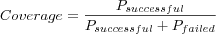
Where
- Psuccessful
is the number of successful predictions (as in a prediction was possible to make) evaluated.
- Pfailed
is the number of failed predictions (as in no prediction could be made).
Keep in mind that it is easy to get 100% coverage, simply implement a RS that makes "default" predictions using some baseline technique (average item rating, average user rating or similar) whenever the "main" prediction fails, however accuracy measures such as MAE may then suffer. While a default prediction is a successful prediction, it is usually more interesting to measure coverage that does not include default predictions
Average User Coverage
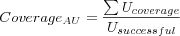
Where
-

is the sum over all user's individual coverage, each user's coverage is calculated as the number of successful predictions made for the user divided by the total number of predictions attempted to be made for the user (e.g. the sum of the number of successful predictions and number of failed predictions for the user).
- Usuccessful
is the number of users evaluated (which does not include users for which no predictions could be made).
Mean Absolute Error (MAE)
Where
- Perror
is the sum of the error for all evaluated predictions, the error in the evaluated predictions is calculated as the absolute value of the difference between the predicted rating PR and the actual rating AR, e.g. |AR-PR|.
- Psuccessful
is the number of successful predictions (as in a prediction was possible to make) evaluated.
Keep in mind the coverage, when coverage goes down (e.g. number of failed predictions increase) less successful predictions will be involved in the MAE calculation, significantly skewing results for the whole test set if coverage is not considered.
MAER using rounded ratings and predictions can also be calculated to better evaluate the user experience.
Average User MAE
Where
-

is the sum over all user's individual MAE, each user's MAE is calculated as the absolute value of the difference between the predicted rating and the actual rating divided with the number of predictions made for the user.
- Usuccessful
is the number of users evaluated (which does not include users for which no predictions could be made).
MAERAU using rounded ratings and predictions can also be calculated to better evaluate the user experience.
Normalized Mean Absolute Error (NMAE)
The MAE for the predictions set is divided with the maximum possible prediction error in order to get a number between 0 and 1 where 0 means all predictions were correct and 1 means all predictions were as wrong as they could possibly be.
 gives the maximum possible MAE, as no prediction error can be larger than the distance between the largest Rmax and smallest Rmin ratings on the rating scale. E.g. suppose actual rating is smallest possible rating 1 and prediction made is largest possible rating 5, then the prediction error is 4 which is also the maximum possible prediction error.
NMAE using rounded ratings and predictions can also be calculated to better evaluate the user experience.
Average User NMAE
Where
-

is the sum over all user's individual NMAE, each user's NMAE is calculated as the user's individual MAE divided by the maximum possible prediction error.
- Usuccessful
is the number of users evaluated (which does not include users for which no predictions could be made).
NMAERAU using rounded ratings and predictions can also be calculated to better evaluate the user experience.
Mean Squared Error (MSE)
Where
-

is the sum of the squared prediction error for all evaluated predictions.
- Psuccessful
is the number of successful predictions (as in a prediction was possible to make) evaluated.
Average User MSE
Where
-

is the sum over all user's individual MSE, each user's MSE is calculated as the user's individual MAE squared.
- Usuccessful
is the number of users evaluated (which does not include users for which no predictions could be made).
MSE using rounded ratings and predictions can also be calculated to better evaluate the user experience.
Root Mean Squared Error (RMSE)

The square root of the MSE for the prediction set is taken to get scaled down error measure where higher values are closer together.
RMSERAU using rounded ratings and predictions can also be calculated to better evaluate the user experience.
Average User RMSE
Where
-

is the sum over all user's individual RMSE, each user's RMSE is calculated as the square root of each user's individual MSE.
- Usuccessful
is the number of users evaluated (which does not include users for which no predictions could be made).
Correctness
Where
- Pcorrect
is the number of rounded predictions that were correct, e.g. matched the known correct rounded rating.
- Psuccessful
is the number of successful predictions (as in a prediction was possible to make) evaluated.
Ranking evaluation metrics
The ranking evaluation metrics measure the RS ability to assemble Top-N ranking lists with known relevant items.
The evaluation metrics assumes that the test user models in the evaluation data consists of items that the user would like to see returned in a Top-N list. For transaction models it is assumed all items are relevant since they were purchased. For rating models it is assumed that since the user rated an item, the user wouldn't have minded seeing it in a Top-N list. Thus the evaluation metrics measure whether the Top-N list contains e.g. movies the user would've shown interest in, not necessarily whether it contains movies the user will like.
In addition to the basic assumption made for evaluating Top-N ranking lists, it can be said that the presence of one known relevant item hopefully gives some credibility to the other items returned in the Top-N lists. Formulated another way, the presence of a relevant item in the Top-N list hopefully increases the probability that the other items in the Top-N list, for which the test model contains no data, are also relevant [McLaughlin & Herlocker, 04].
It would also be possible to consider only the items the user has rated highly as relevant and treat those not rated highly as non-rated (they become part of the set of items not rated by the user). This can be accomplished by using a rating threshold and treat items rated equal to or above the rating threshold as relevant. The rating threshold can either be global for all users or possibly be individual for each user (e.g. use the user's mean rating).
Alternatively items below the rating threshold could be considered as known non-relevant instead of being treated as non-rated. By the same assumptions made for the presence of known relevant items, it is possible to then check for the presence of known non-relevant items (this is not the same as unrated items). The presence of known non-relevant items would then indicate a bad Top-N list. Similarly it can also be assumed that the presence of a known non-relevant item in a Top-N list most likely increases the likelihood that the other items in the Top-N list, for which the test model contains no data, are also non-relevant.
Evaluations considering only items with ratings above (or as suggested below) a rating threshold, are made by using training/test data sets where the test data only consists of ratings meeting the rating threshold. Note that it makes little sense to include in the test rating data items that are known non-relevant if those items are just ignored during the evaluation. While it would be possible to use a test model consisting of both known relevant and known non-relevant items and at evaluation time check for the presence of both in the Top-N list, the only way to measure the accuracy of such a system using the common evaluation metrics presented in this paper, would still be by measuring independently recall and precision of known relevant and known non-relevant items. That said, it might be interesting to attempt a accuracy measure that simultaneously checks for the presence of known relevant and known non-relevant items. (E.g. what exactly does it mean that recall is 20% for known relevant items and 20% for non-relevant items?)
Another alternative to evaulating ranking lists is to within a given Top-N list consider only the rated items and ignore the non rated items during evaluation, this would however lead to underestimates and will not be considered further. (E.g. in a Top-100 list, perhaps only 4 items have been rated by the user, two favourably and two negatively, ignoring non-rated items would give e.g. a precision of 2/4=50%, while treating non-rated as non-relevant and rated as relevant would give a precision of 4/100=4%.)
In addition to reporting the metrics described in this section, it is important to also report how many users could be evaluated (successful users) and how many users could not be evaluated (failed user). Additionally number of evaluated users with no relevant items returned and average size of Top-N ranking list can be reported [Table 8].
| Usuccessful | Number of successful users evaluated (excluding users for which no recommendations could be made, but including users with Top-N lists containing no relevant items). |
| Ufailed | Number of failed users that could not be evaluated (Top-N list empty, no recommendations at all was possible for the user). |
| TNsuccessful | Number of successful Top-N lists (as in contains at least one relevant item). |
| TNfailed | Number of failed Top-N lists (as in contains no relevant items, includes empty Top-N lists). |
| TNa | Average size of Top-N ranking list. Expected to be N, but may be less if N recommendations is not possible for all users. |
additional ranking metrics
Coverage
Where
- TNsuccessful
is the number of successful Top-N lists (as in contains at least one relevant item).
- TNfailed
is the number of failed Top-N lists (as in contains no relevant items, includes empty Top-N lists).
Recall
Where
- RIreturned
is the total number of relevant items returned over all users.
- RI
is the total number of known relevant items that could have been returned.
Note that the size of the Top N ranking list might make it impossible to get a perfect recall, e.g. N=10 but user has rated 2000 items making it impossible to recall all relevant items. However recall relates to precision, and precision typically goes down if we increase recall, hence a perfect recall isn't always wanted, but a good balance between recall and precision typically is.
Average User Recall
Where
-

is the sum over all users of each users individual recall, which is the number of returned relevant items in the user's Top-N list divided by the total number of known relevant items (or n if number of known items exceeds n in order to only evaluate if what could possibly be returned was returned).
- Usuccessful
is the number of successful users evaluated (excluding users for which no recommendations could be made, but including users with Top-N lists containing no relevant items).
The max number of known relevant items that can be recalled for the user is thus equal to the size of the user's test data set and the size of the Top-N list, do not go by the size of the test data set as it might contain more than n items, in which case a perfect recall will never be achieved and measurement would be skewed towards smaller recall data sets.
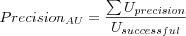
Precision
Where
- RIreturned
is the total number of relevant returned items over all users.
- Ireturned
is the total number of returned items over all users.
Precision tells us how many of the returned items are known to be relevant, however keep in mind that we are not working with complete data, we do not know of all items that are relevant to the user, hence precision is not wanted to be perfect.
Average User Precision
Where
-

is the sum over all users of each users individual precision, which is the user's recall divided with the number of items returned in the users Top-N list (which is less than or equal to n in order to not skew results towards small test sets that can fit in the Top-N list).
- Usuccessful
is the number of successful users evaluated (excluding users for which no recommendations could be made, but including users with Top-N lists containing no relevant items).
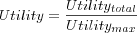
(Breeze's / Halflife) Utility
Where
- Utilitytotal
is the sum over all users of each user's individual utility Ra , where Ra is defined by Breeze as:
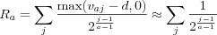
Where j is the position (starting at 1) in the Top-N list of a relevant item. The constant a , called the halflife constant, is a guess of which position in the Top-N list there is a 50% chance of user looking at.
The summation is over relevant items in the Top-N list, relevant items in early positions in the Top-N list have a high utility for the user, whereas items further down have a lower utility as the user isn't as likely to view those. Non relevant items serve to push relevant items further down the Top-N list, thus decreasing the utility of the relevant items in the Top-N list. The choice of a is made heuristically, the idea is that a user isn't likely to look at the 100th item in a top 100 list, however the first 5 are very likely to be viewed, hence 5 might be a suitable halflife constant. Breeze uses 5 [Breese et al., 98].
The term
 , with vaj denoting user a's rating (Breeze calls them votes) on item j , causes items with ratings below what Breeze calls the "default vote" d to be ignored. Assuming a rating scale of 1-5 the constant d can be chosen to be the middle of the rating scale, e.g. 3, in which case items a user has rated with 1,2 or 3 would be ignored and not increase the utility if encountered in the Top-N list. However, the idea of a "default vote" is impractical (not all system makes "default votes") as well as not very meaningful. Ignoring the ratings all together makes more sense, since it was initially stated that the evaluation is based on the assumption the user model only contains relevant items. A low rating doesn't indicate a lower relevance by that assumption. Thus it is motivated to replace the term
  with 1 to simplify the formula and make it more understandable and useable for both rating and transaction data. With this new formulation the utility of the item at the "halflife" position is always 0.5.
Unless otherwise noted the simplified version of Breeze's utility will be used.
- Utilitymax
is the sum over all users of each users individual max utility Rm , where Rm is defined as:

Where j goes from 1 to number of known relevant items or the size of the Top-N list. E.g. the maximum utility is achieved when either all known relevant items are at the top of the user's Top-N list, or when the entire Top-N list consists of known relevant items.
Average User (Breeze's / Halflife ) Utility
Where
-

is the sum over all users of each user's individual utility, which is the user's utility divided with the user's max utility.
- Usuccessful
is the number of successful users evaluated (excluding users for which no recommendations could be made, but including users with Top-N lists containing no relevant items).
F1
Since recall and precision complement each other, e.g. low recall typically occurs with high precision, and low precision occurs with high recall, both measures tell more about the situation than one alone, the F1 metric thus aims to combine both measures to get a accuracy metric of higher quality. A high value of the F1 metric ensurse that both precision and recall was reasonably high.
Average User F1
Where
-

is the sum over all users of each user's individual F1.
- Usuccessful
is the number of successful users evaluated (excluding users for which no recommendations could be made, but including users with Top-N lists containing no relevant items).
Average First Hit Position
Where
-

is the sum over all users position of their first relevant item (users with no relevant items returned have no first relevant item and are thus ignored).
- Usuccessful
is the number of successful users evaluated (excluding users for which no recommendations could be made, but including users with Top-N lists containing no relevant items).
Evaluation data
Evaluations will be made based on four datasets. Three rating datasets and one transaction dataset. Each dataset is represent by a set of histograms showing some characteristics of the datasets. Comparison of the histograms reveals common characteristics between the rating datasets, such as a normal distribution of ratings etc.
Consistent MovieLens rating dataset (CML)
The 100.000 ratings MovieLens rating dataset was collected by the GroupLens Research Project at the University of Minnesota. The dataset consists of user ratings on movies, ratings are on a 1-5 scale ("half-star" ratings were later introduced into their experimental movie recommender system.)
The original rating dataset contained a few inconsistencies that was removed, in particular 20 pairs of movies with different "id" are really the same movies, meaning users have rated the same movie twice. These inconsistencies were resolved by removing one of the movies and keeping each user's higher rating in the cases a user had rated both movies and differently. Four movies in the set that could not be located in the IMDb were also removed as we needed to be able to retrieve attribute data for all movies. This lead to a reduction of 24 items and 304 ratings, no users needed to be removed. The rating dataset still consists of only users that have rated at least 20 movies (with the exception of one user that now only has 19 ratings). All movies in the dataset we used contain IMDb ids, meaning we could use the publicly available IMDb attribute datasets together with the rating dataset.
Statistics for the rating dataset are shown in [cml statistics] .
| Users | 943 |
| Items | 1658 |
| Ratings | 99696 |
| Sparsity (of user-item matrix) | 93% |
| Mean rating (for users) | 3.53 |
| Average number of ratings per user | 105 |
| Average number of ratings per item | 60 |
cml statistics
Sparsity is quite high, however this is to be expected for any dataset as users and items increase and is part of the challenge of recommender systems based on rating data. The number of users and items is relatively small, however the dataset is used in many papers and is thus still interesting to include. A large MovieLens rating dataset consisting of 1 million ratings is also offered, however we chose to only work with this smaller dataset. Naturally the hope is that results on this dataset give a good hint of results on larger datasets, whether or not that is the case is hard to know.
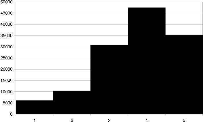
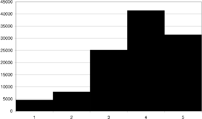
If we look at a histogram showing how often the discrete ratings 1-5 are used we see that the spread is roughly normal distributed [cml rating fq] .
cml rating fq Histogram showing the rating frequency in the CML dataset, i.e. how many times each discrete grade 1-5 is assigned an item.
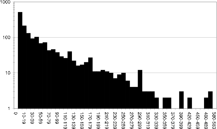
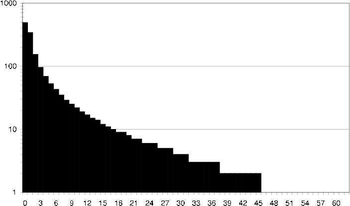
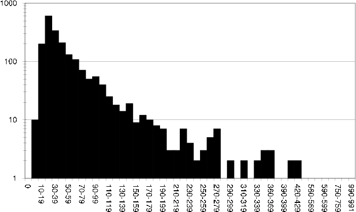
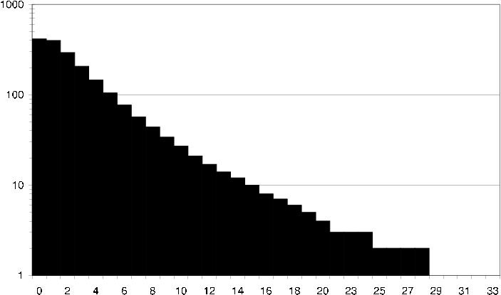
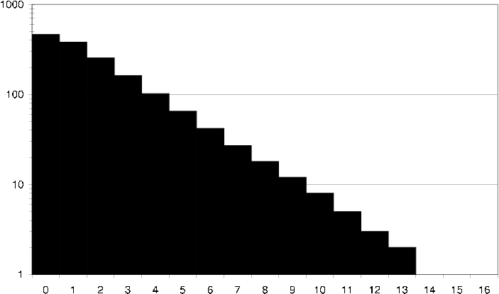
The average number of ratings per user is 105, if we look at a histogram showing how many users have rated varying numbers of items we get a better idea of the rating spread [cml user rating fq] .
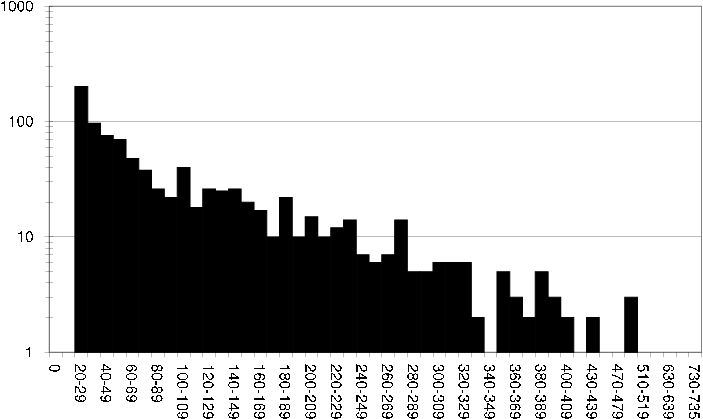
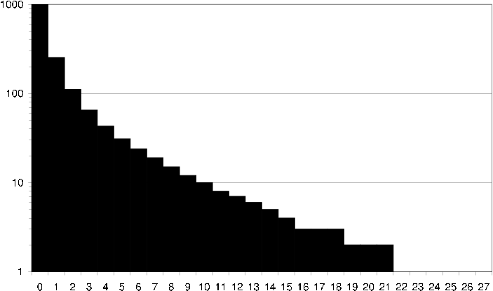
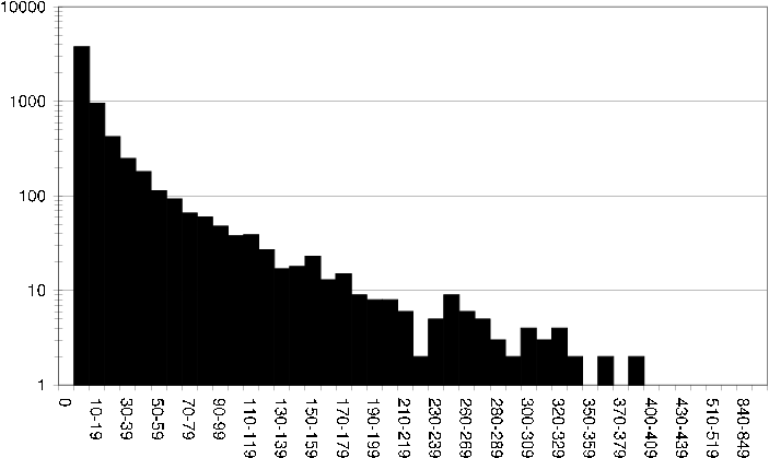
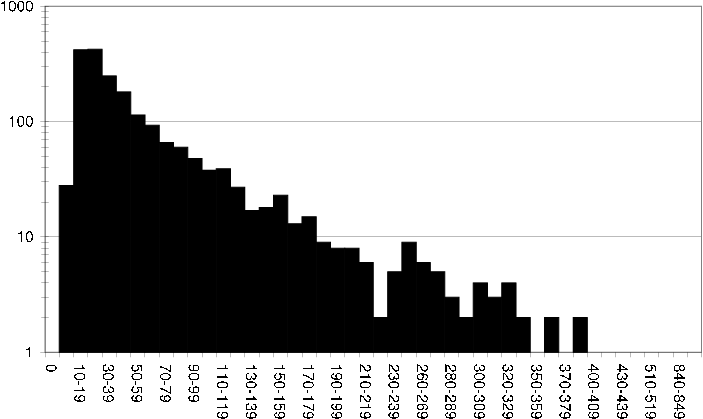
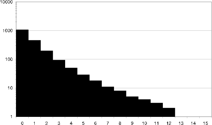
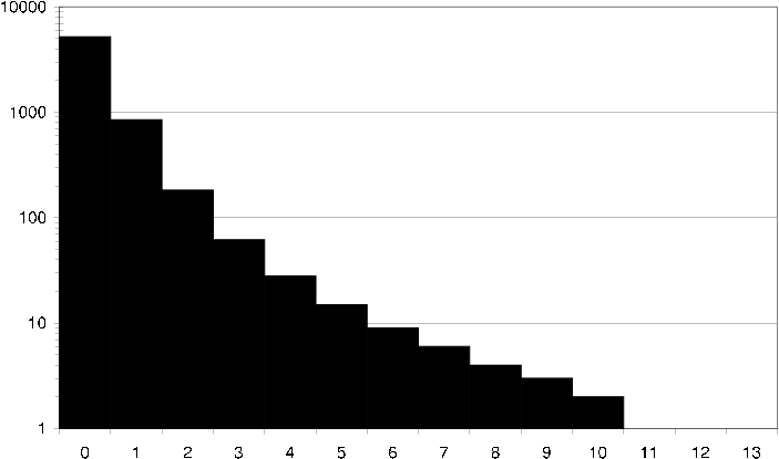
Similarly we can look closer at the per item rating spread, which is relevant in item based recommendation techniques that will use this rating data [cml item rating fq] .
cml user rating fq Histogram showing how many users have rated varying numbers of items in the CML dataset.
cml item rating fq Histogram showing how often items have been rated in the CML dataset.
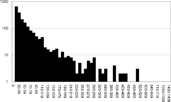
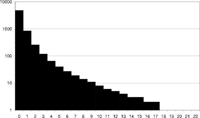
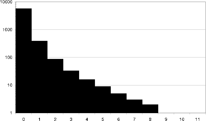
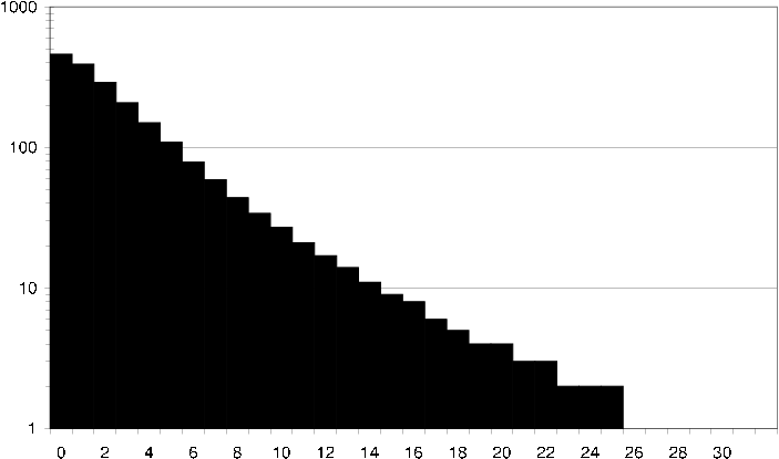
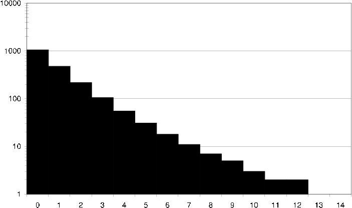
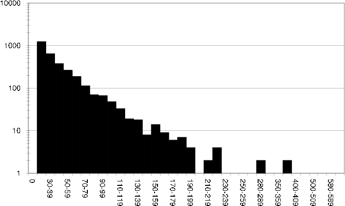
Interesting to study is also how an average user relates to its neighbors. I.e. given any user in the rating dataset, how many neighbors does the user have 100 items in common with [cml average user common items] , and how many neighbors does the user have 100 items in common with that are rated the same [cml average user common ratings] .
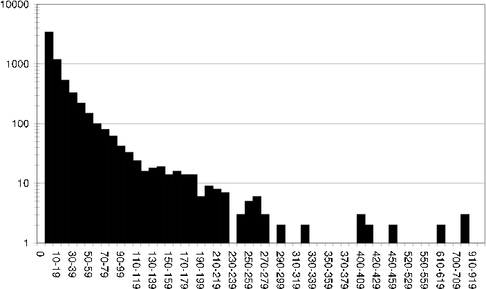
Similarly it is interesting to study how an average item relates to its neighbors. I.e. given any item in the rating dataset, how many neighbors does the item have 100 users in common with [cml average item common users] , and how many neighbors does the item have 100 users in common with that have assigned the item and the neighbor the same rating [cml average item common ratings] .
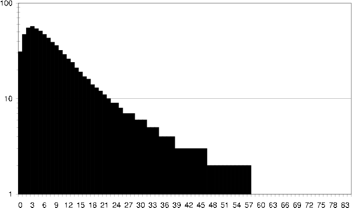
cml average user common items How an average user in the CML dataset relates to its neighbors in terms of common items. I.e. how many neighbors does the user have exactly 40 items in common with?
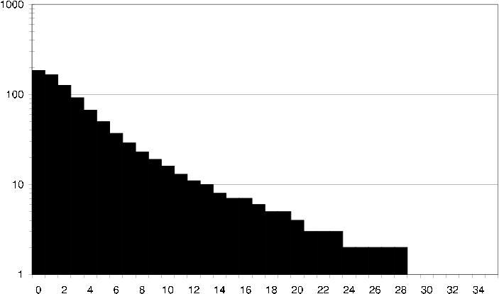
cml average user common ratings How an average user in the CML dataset relates to its neighbors in terms of common ratings. I.e. how many neighbors does the user have exactly 10 items in common with that both the user and the neighbor have rated the same.
cml average item common users How an average item in the CML dataset relates to its neighbors in terms of common users. I.e. how many neighbors does the item have exactly 40 users in common with?
cml average item common ratings How an average item in the CML dataset relates to its neighbors in terms of common ratings. I.e. how many neighbors does the item have exactly 10 users in common with that have given the item and its neighbor the same rating.
Discshop rating dataset (DS)
Dataset consists of ratings collected from a Swedish e-commerce site selling DVDs.
Dataset is a preprocessed version of a larger dataset. In particular the original dataset consisted of user ratings on products instead of directly on movies. E.g. ratings were assigned per DVD edition of a movie. When rating a DVD edition the customer was allowed to assign multiple grades, in particular one grade to the DVD edition and one grade to the movie itself. A user may thus rate different DVD editions of the same movie and in the process the user might give the same movie different ratings, this may occur because user changed opinion about the movie or because DVD edition contain significantly different cuts of the movie. The original rating dataset on products does not allow for discerning between different cuts of the same movie, a movie is always the same movie independent of the cut. E.g. Blade Runner and Blade Runner Directors Cut is both identified as the movie Blade Runner, though with two different DVD editions. In order to create this rating dataset of movies, products were mapped to movies by keeping the grade assigned to the movie and ignoring the grade assigned to the DVD edition. In the cases a user had rated multiple DVD editions of the same movie, the highest grade assigned the movie was kept. The reason for not working with the ratings of DVD editions was made in order to get a simpler dataset to work with, a dataset that can easily be used together with attribute datasets for movies.
It was considered practical to ignore users with less than 20 rated movies. Any recommendation technique is considered unlikely to be able to produce reliable recommendations based on too little information about users, in this case less than 20 ratings was considered too little information. By ignoring users with few ratings the size of the rating dataset was also reduced to a more manageable size. Statistics for the rating dataset are shown in [ds statistics] .
| Users | 2001 |
| Items | 6256 |
| Ratings | 129829 |
| Sparsity (of user-item matrix) | 98% |
| Mean rating (for users) | 3.74 |
| Average number of ratings per user | 64 |
| Average number of ratings per item | 20 |
ds statistics
If we look at a histogram showing the distribution of ratings, we see that it is very similar to the distribution for the CML dataset [ds rating fq] .
ds rating fq Histogram showing the rating frequency in the DS dataset, i.e. how many times each discrete grade 1-5 is assigned to an item.
The average number of ratings per user is 64 in the DS dataset, if we look at a histogram showing how many users have rated varying numbers of items we get a better idea of the rating spread [ds user rating fq] .
Similarly we can look closer at the per item rating spread, which is relevant in item based recommendation techniques that will use this rating data [ds item rating fq] .
ds user rating fq Histogram showing how many users have rated varying numbers of items in the DS dataset.
ds item rating fq Histogram showing how often items have been rated in the DS dataset.
Interesting to study is also how an average user relates to its neighbors. I.e. given any user in the rating dataset, how many neighbors does the user have 100 items in common with [ds average user common items] , and how many neighbors does the user have 100 items in common with that are rated the same [ds average user common ratings] . Similarly it is interesting to study how an average item relates to its neighbors. I.e. given any item in the rating dataset, how many neighbors does the item have 100 users in common with [ds average item common users] , and how many neighbors does the item have 100 users in common with that have assigned the item and the neighbor the same rating [ds average item common ratings] .

ds average user common items How an average user in the DS dataset relates to its neighbors in terms of common items. I.e. how many neighbors does the user have exactly 40 items in common with?

ds average user common ratings How an average user in the DS dataset relates to its neighbors in terms of common ratings. I.e. how many neighbors does the user have exactly 10 items in common with that both the user and the neighbor have rated the same.
ds average item common users How an average item in the DS dataset relates to its neighbors in terms of common users. I.e. how many neighbors does the item have exactly 40 users in common with?
ds average item common ratings How an average item in the DS dataset relates to its neighbors in terms of common ratings. I.e. how many neighbors does the item have exactly 10 users in common with that have given the item and its neighbor the same rating.
Discshop rating dataset 2 (DS2)
Dataset is a subset of the DS dataset in which it has been required that in addition to each user having to have rated at least 20 items, each item must also have been rated by 20 users. This avoids situations in which a user has indeed rated 20 items, but that user is the only user that has rated those items. The enforcement is for simplicity not strict, some items will be rated by less than 20 users, however most of the items will have been rated by more than 20 users.
Statistics for the rating dataset are shown in [ds2 statistics] .
| Users | 2001 |
| Items | 1962 |
| Ratings | 110418 |
| Sparsity (of user-item matrix) | 97% |
| Mean rating (for users) | 3.79 |
| Average number of ratings per user | 55 |
| Average number of ratings per item | 56 |
ds2 statistics
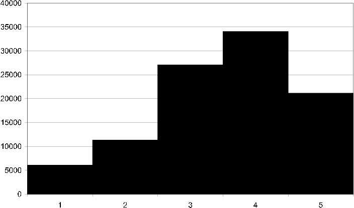
If we look at a histogram showing how often the discrete ratings 1-5 are used we see that the spread is roughly normal distributed [ds2 rating fq] and similar to the DS data's rating spread.
ds2 rating fq Histogram showing the rating frequency in the DS2 dataset, i.e. how many times each discrete grade 1-5 is assigned an item.
The average number of ratings per user is 55, if we look at a histogram showing how many users have rated varying numbers of items we get a better idea of the rating spread [ds2 item rating fq] .
Similarly we can look closer at the per item rating spread, which is relevant in item based recommendation techniques that will use this rating data [ds2 user rating fq] .
ds2 user rating fq Histogram showing how many users have rated varying numbers of items in the DS2 dataset.
ds2 item rating fq Histogram showing how often items have been rated in the DS2 dataset.
Interesting to study is also how an average user relates to its neighbors. I.e. given any user in the rating dataset, how many neighbors does the user have 100 items in common with [ds2 average user common items] , and how many neighbors does the user have 100 items in common with that are rated the same [ds2 average user common ratings] . Similarly it is interesting to study how an average item relates to its neighbors. I.e. given any item in the rating dataset, how many neighbors does the item have 100 users in common with [ds2 average item common users] , and how many neighbors does the item have 100 users in common with that have assigned the item and the neighbor the same rating [ds2 average item common ratings] .
ds2 average user common items How an average user in the DS2 dataset relates to its neighbors in terms of common items. I.e. how many neighbors does the user have exactly 40 items in common with?
ds2 average user common ratings How an average user in the DS2 dataset relates to its neighbors in terms of common ratings. I.e. how many neighbors does the user have exactly 10 items in common with that both the user and the neighbor have rated the same.
ds2 average item common users How an average item in the DS2 dataset relates to its neighbors in terms of common users. I.e. how many neighbors does the item have exactly 40 users in common with?
ds2 average item common ratings How an average item in the DS2 dataset relates to its neighbors in terms of common ratings. I.e. how many neighbors does the item have exactly 10 users in common with that have given the item and its neighbor the same rating.
Discshop transaction dataset (DS-T)
In addition to the rating dataset we also obtain a transaction dataset. Dataset consists of user (customer) transactions. A transaction in this case is defined as a purchase by a user of a single item (movie). Dataset does not aid in market basket analysis as a users complete purchase history has been aggregated. All users in the dataset have purchased at least 20 movies.
Statistics for the transaction dataset are shown in [dst statistics] .
| Users | 3158 |
| Items | 6380 |
| Transactions | 145637 |
| Sparsity (of user-item matrix) | 99% |
| Average number of transactions per user | 46 |
| Average number of transactions per item | 22 |
dst statistics
Histograms showing the per user and item purchase distribution are shown in [Figure 37,Figure 38], as well as an average user and average items relation to its neighbors in [Figure 39,Figure 40].
dst user transaction size Histogram showing the distribution of the size of user transactions in the DS-T dataset.
dst item transaction size Histogram showing the distribution of the size of item transactions in the DS-T dataset.
dst average user common transactions How an average user in the DS-T dataset relates to its neighbors in terms of common transactions. I.e. how many neighbors does the user have exactly 40 purchased items in common with?
dst average item common transactions How an average item in the DS-T dataset relates to its neighbors in terms of common transactions. I.e. how many neighbors does the item have exactly 40 users (i.e. users that have purchased both the item and the neighbor) in common with?
Discshop attribute dataset (DS-A)
In addition to the movie rating- and movie transaction- data we also obtain the information displayed for the movies the customers could purchase, we prepare this per movie attribute information into separate datasets consisting of one type of attribute each. The attribute types we will work with are:
Actor
Age limit
Country
Director
Genre
Title
Alternative title
Original title
Writer
Year
IMDb attribute dataset (IMDB)
The movie attribute dataset are obtain from The Internet Movie Database (IMDb). The original attribute datasets use the movie's original title as key, movies with the same title have a identifier specifying the duplication number appended. However, for our purposes it turns out to be more practical to work with IMDb Constant Title Codes ("IMDb-ids"), especially as the CML dataset has been converted to use IMDb-ids. Thus we prepared IMDb attribute datasets that use IMDb-ids instead of the unique IMDb movie titles.
We prepared datasets consisting of one attribute type each, the attribute types we will work with are:
Actors
Actresses
Cinematographers
Color info
Composers
Costume designers
Countries
Directors
Distributors
Editors
Genres
Keywords
Language
Locations
Miscellaneous companies
Miscellaneous
Producers
Production companies
Production designers
Sound-mix
Special effects companies
Technical
Title
Writers
Evaluation results
The recommendation techniques were evaluated for the evaluation datasets using various combinations of evaluation protocol, training/test data formation and evaluation metrics.
For the recommendation techniques we select where necessary an appropriate combination of similarity and prediction algorithm, we use a decent set of settings giving good results, not necessarily the absolute best results, but near enough to be interesting to list.
We will describe briefly for each recommendation technique the setup of the evaluation, such that the evaluation can easily be understood and reproduced.
Accuracy of predictions
The result tables use the following abbreviations for the column headings: ET = Total evaluation time, Us = Usuccessful , Uf = Ufailed , Ps = Psuccessful , Pf = Pfailed , Cov = Coverage, Corr = Correctness, P = Precision.
The settings column names the recommendation algorithm instance used of the recommendation technique in question. Typically only the name of the dataset used for evaluation is given (i.e. DS, DS2 or CML). Each table of evaluation results is followed by a description of algorithms and settings used for each recommendation technique.
In all cases a 10-fold evaluation as previously described was performed. Note that the same 10-folded evaluation data of each dataset were used for each evaluation.
BASELINESF Technique
| Settings | ET | Us | Uf | Ps | Pf | Cov | Corr | MAE | MAER | MAEUA | MAERUA | NMAE | MSE | RMSE |
| DS-UM | 0 | 2001 | 0 | 12982 | 0 | 100.0% | 39.7% | 0.780 | 0.745 | 0.804 | 0.771 | 0.195 | 1.001 | 1.001 |
| DS-IM | 0 | 2000 | 0 | 12861 | 121 | 99.1% | 41.8% | 0.760 | 0.720 | 0.778 | 0.739 | 0.190 | 0.965 | 0.983 |
| DS-PDFM | 0 | 2000 | 0 | 12861 | 121 | 99.1% | 46.0% | 0.687 | 0.649 | 0.700 | 0.665 | 0.172 | 0.820 | 0.906 |
| DS-R | 0 | 2001 | 0 | 12982 | 0 | 100.0% | 21.1% | 1.428 | 1.429 | 1.482 | 1.483 | 0.357 | 3.047 | 1.746 |
| DS2-UM | 0 | 1991 | 0 | 11035 | 0 | 100.0% | 40.3% | 0.766 | 0.730 | 0.792 | 0.760 | 0.192 | 0.968 | 0.984 |
| DS2-IM | 0 | 1991 | 0 | 11035 | 0 | 100.0% | 42.9% | 0.736 | 0.694 | 0.764 | 0.723 | 0.184 | 0.898 | 0.948 |
| DS2-PDFM | 0 | 1991 | 0 | 11035 | 0 | 100.0% | 47.2% | 0.667 | 0.627 | 0.688 | 0.651 | 0.167 | 0.772 | 0.879 |
| DS2-R | 0 | 1991 | 0 | 11035 | 0 | 100.0% | 21.1% | 1.435 | 1.435 | 1.488 | 1.487 | 0.359 | 3.078 | 1.754 |
| CML-UM | 0 | 943 | 0 | 9967 | 0 | 100.0% | 36.2% | 0.834 | 0.802 | 0.842 | 0.809 | 0.209 | 1.084 | 1.041 |
| CML-IM | 0 | 943 | 0 | 9952 | 15 | 99.8% | 36.9% | 0.815 | 0.783 | 0.833 | 0.801 | 0.204 | 1.043 | 1.021 |
| CML-PDFM | 0 | 943 | 0 | 9952 | 15 | 99.8% | 40.8% | 0.754 | 0.718 | 0.776 | 0.742 | 0.189 | 0.916 | 0.957 |
| CML-R | 0 | 943 | 0 | 9967 | 0 | 100.0% | 21.7% | 1.386 | 1.385 | 1.400 | 1.399 | 0.346 | 2.875 | 1.695 |
baselinesf prediction accuracy
As a statistical prediction algorithm the PDFM algorithm seems to be the one that gives the lowest MAE for both datasets. Note that neither of the algorithms are truly CF algorithms, though they rely on the same rating datasets as the CF algorithms we will later try and thus serves as a decent statistical baseline to compare CF algorithms performance against. The results of the random prediction algorithm can be seen to serve as a comparison against any prediction algorithm, as the aim is at least to be better than a random prediction algorithm in any circumstance.
UCF Technique
| Settings | ET | Us | Uf | Ps | Pf | Cov | Corr | MAE | MAER | MAEUA | MAERUA | NMAE | MSE | RMSE |
| DS | 3 | 1990 | 10 | 12729 | 253 | 98.0% | 47.2% | 0.679 | 0.640 | 0.701 | 0.664 | 0.170 | 0.820 | 0.906 |
| DS2 | 2 | 1978 | 12 | 11002 | 33 | 99.7% | 48.2% | 0.657 | 0.618 | 0.687 | 0.652 | 0.164 | 0.768 | 0.876 |
| CML | 1 | 943 | 0 | 9952 | 15 | 99.8% | 42.7% | 0.729 | 0.692 | 0.753 | 0.718 | 0.182 | 0.874 | 0.935 |
ucf prediction accuracy
Since the UCF technique sorts neighbors in descending order of similarity (highest first) it means that the 30 most similar neighbors to the active user were used as recommenders. We can note that the technique in this case performs better for both datasets than the best performing instance of the baseline technique in terms of MAE.
RNUCF Technique
| Settings | ET | Us | Uf | Ps | Pf | Cov | Corr | MAE | MAER | MAEUA | MAERUA | NMAE | MSE | RMSE |
| DS | 4 | 2000 | 0 | 12861 | 121 | 99.1% | 45.8% | 0.692 | 0.653 | 0.704 | 0.668 | 0.173 | 0.829 | 0.911 |
| DS2 | 1 | 1991 | 0 | 11035 | 0 | 100.0% | 46.7% | 0.672 | 0.633 | 0.692 | 0.656 | 0.168 | 0.783 | 0.885 |
| CML | 1 | 943 | 0 | 9952 | 15 | 99.8% | 40.5% | 0.762 | 0.726 | 0.784 | 0.749 | 0.190 | 0.934 | 0.967 |
rnucf prediction accuracy
Exactly the same settings and algorithms as in the UCF Technique evaluation were used. However since the RNUCF technique unlike the UCF technique (to which it otherwise is identical) sorts neighbors randomly it means that between 1 and 30 randomly chosen neighbors will be used as recommenders. Note that only neighbors with which a similarity could be calculated will be considered. So this truly is a random neighbors version of the UCF technique. We can note that the technique in this case only performs marginally worse than the UCF technique for both datasets in terms of MAE. Can this be a consequence of most similarities being observed to be very low, and as such any similarity will do as good as any other?
TRUSTUCF Technique
| Settings | ET | Us | Uf | Ps | Pf | Cov | Corr | MAE | MAER | MAEUA | MAERUA | NMAE | MSE | RMSE |
| DS | 16 | 1969 | 31 | 10888 | 2094 | 83.9% | 47.4% | 0.676 | 0.639 | 0.700 | 0.666 | 0.169 | 0.820 | 0.906 |
| DS2 | 11 | 1963 | 27 | 10288 | 747 | 93.2% | 47.9% | 0.664 | 0.627 | 0.693 | 0.659 | 0.166 | 0.793 | 0.890 |
| CML | 6 | 942 | 0 | 9583 | 384 | 96.1% | 42.9% | 0.733 | 0.695 | 0.759 | 0.723 | 0.183 | 0.892 | 0.944 |
trustucf prediction accuracy
Again the same settings and algorithms as in the UCF Technique evaluation were used. However the similarity between the active user and the active user's neighbors is weighted depending on how much the neighbors are trusted to be able to predict for the active item. We can note that the technique in this case performs basically equally well as the UCF technique for both datasets in terms of MAE. Coverage is however lower than for the UCF technique.
CIPUCF Technique
| Settings | ET | Us | Uf | Ps | Pf | Cov | Corr | MAE | MAER | MAEUA | MAERUA | NMAE | MSE | RMSE |
| DS | 5 | 1990 | 10 | 12729 | 253 | 98.0% | 46.7% | 0.684 | 0.645 | 0.711 | 0.674 | 0.171 | 0.826 | 0.909 |
| DS2 | 3 | 1978 | 12 | 11002 | 33 | 99.7% | 47.7% | 0.663 | 0.624 | 0.697 | 0.662 | 0.166 | 0.774 | 0.880 |
| CML | 1 | 943 | 0 | 9952 | 15 | 99.8% | 42.7% | 0.733 | 0.696 | 0.758 | 0.724 | 0.183 | 0.887 | 0.942 |
cipucf prediction accuracy
Again the same settings and algorithms as in the UCF Technique evaluation were used. However neighbors with most items common with the active user were prioritized in hopes of those similarities being most reliable. We can note that the technique in this case only performs marginally worse than the UCF technique for both datasets in terms of MAE.
ICF Technique
| Settings | ET | Us | Uf | Ps | Pf | Cov | Corr | MAE | MAER | MAEUA | MAERUA | NMAE | MSE | RMSE |
| DS | 10 | 1998 | 2 | 12591 | 391 | 97.0% | 43.9% | 0.727 | 0.690 | 0.776 | 0.745 | 0.182 | 0.917 | 0.958 |
| DS2 | 2 | 1990 | 0 | 11033 | 2 | 100.0% | 44.6% | 0.707 | 0.669 | 0.764 | 0.731 | 0.177 | 0.861 | 0.92 |
| CML | 1 | 943 | 0 | 9936 | 30 | 99.7% | 41.7% | 0.744 | 0.708 | 0.786 | 0.751 | 0.186 | 0.902 | 0.950 |
icf prediction accuracy
Since the ICF technique sorts item neighbors (items similar to the active item) in descending order of similarity (highest first) it means that the 30 most similar items that the active user had rated were used as a basis for the predictions. We can note that the technique in this case for all datasets performs worse than or equal to the best performing instance of the baseline technique in terms of MAE.
RNICF Technique
| Settings | ET | Us | Uf | Ps | Pf | Cov | Corr | MAE | MAER | MAEUA | MAERUA | NMAE | MSE | RMSE |
| DS | 11 | 1999 | 1 | 12858 | 124 | 99.0% | 40.0% | 0.786 | 0.750 | 0.807 | 0.773 | 0.196 | 1.031 | 1.015 |
| DS2 | 1 | 1991 | 0 | 11035 | 0 | 100.0% | 40.2% | 0.772 | 0.735 | 0.795 | 0.763 | 0.193 | 0.984 | 0.992 |
| CML | 0 | 943 | 0 | 9952 | 15 | 99.8% | 36.0% | 0.843 | 0.811 | 0.847 | 0.815 | 0.211 | 1.109 | 1.053 |
rnicf prediction accuracy
Exactly the same settings and algorithms as in the ICF Technique evaluation were used. However since the RNICF technique unlike the ICF technique (to which it otherwise is identical) sorts item neighbors randomly it means that between 1 and 30 randomly chosen item will be used as neighbors for the active item and make the basis for the predictions. Note that only neighbors with which a similarity could be calculated will be considered. So this truly is a random neighbors version of the ICF technique. We can note that the technique in this case only performs somewhat worse than the ICF technique for both datasets in terms of MAE. The evaluation based on the CML dataset seems to do a bit more than worse though compared to the ICF technique.
PCBF Technique
| Settings | ET | Us | Uf | Ps | Pf | Cov | Corr | MAE | MAER | MAEUA | MAERUA | NMAE | MSE | RMSE |
| DS | 42 | 2001 | 0 | 12975 | 7 | 99.9% | 41.3% | 0.758 | 0.722 | 0.788 | 0.755 | 0.190 | 0.958 | 0.979 |
| DS2 | 22 | 1990 | 0 | 11029 | 6 | 99.9% | 41.9% | 0.746 | 0.709 | 0.777 | 0.741 | 0.186 | 0.930 | 0.965 |
| CML | 7 | 943 | 0 | 9935 | 32 | 99.7% | 38.3% | 0.790 | 0.756 | 0.809 | 0.777 | 0.197 | 0.982 | 0.99 |
pcbf prediction accuracy
For the DS dataset six different attribute types from the DS-A dataset were used: Actor, Age limit, Country, Director, Writer and Genre. The Common Attributes similarity algorithm were used for the Actor, Age limit, Country and Writer attribute types. The Attribute Cosine similarity algorithm were used for the Director and Genre attribute types. For both similarity algorithms (in all cases) at least one common attribute was required and a significance threshold of 30 was used (which might not be a good choice seeing how movies only for the actor attribute type is likely to have more than 30 attributes). Similarities were weighted based on which attribute they were based on as follows; Actor 10, Age limit 1, Country 3, Director 9, Genre 8 and Writer 9 (e.g. the Actor similarity makes up  of the total similarity). That is, actors, director, genre and write were most influential while age limit and country influence the final similarity very little. For the CML dataset all available attribute types except title in the IMDB dataset were used, again the Common Attributes and Attribute Cosine similarity algorithms were used with the same settings as for the DS dataset. Varying weights were used for the different attributes, highest influence was placed on similarities based on the Actor, Actress, Director, Writer and Genre attribute types. The Weighted Sum prediction algorithm was used to generate predictions, basing its predictions on a neighborhood consisting of at least 1 neighbor and at most 30 neighbors. Complete item similarly models were generated, i.e. for each item its similarities with all other items were precalculated and available for consideration by the prediction algorithm.
We can note that the technique in this case only performs somewhat worse than the ICF technique for both datasets in terms of MAE, it performs marginally better than the RNICF technique however.
Relevance of Top-N ranking lists
The result tables use the following abbreviations for the column headings: ET = Total evaluation time, Us = Usuccessful , Uf = Ufailed , TNs = TNsuccessful , TNf = TNfailed , Cov=Coverage, R=Recall, P=Precision, U=Utility, RAU = RecallAU , PAU = PrecisionAU , UAU = UtilityAU .
In all cases, unless otherwise noted, a 10-fold evaluation was performed. Note that the same 10-folded datasets were used for each evaluation.
In all cases a top N=10 list was generated for each user. When measuring the utility the half life constant a was set to 5 in all cases.
TOPNUCF Technique
| Settings | ET | Us | Uf | TNs | TNf | TNa | Cov | R | P | F1 | U | AFHP | RAU | PAU | F1AU | UAU |
| CML | 47 | 943 | 0 | 310 | 632 | 10 | 32.9% | 4.6% | 4.8% | 0.047 | 0.042 | 4 | 4.5% | 4.8% | 0.039 | 0.038 |
| DS (4 Fold w/ 75% Test) | 8 | 495 | 1505 | 421 | 1579 | 6 | 21.1% | 2.6% | 40.8% | 0.049 | 0.078 | 1 | 3.1% | 41.5% | 0.057 | 0.078 |
| DS2 (4 Fold w/ 75% Test) | 33 | 1968 | 29 | 572 | 1426 | 9 | 28.6% | 2.7% | 3.7% | 0.031 | 0.031 | 4 | 3.2% | 3.8% | 0.031 | 0.030 |
| CML (4 Fold w/ 75% Test) | 3 | 761 | 181 | 688 | 254 | 9 | 73.0% | 3.6% | 36.3% | 0.065 | 0.063 | 2 | 4.5% | 36.6% | 0.075 | 0.063 |
topnucf ranking relevance
TOPNICF Technique
| Settings | ET | Us | Uf | TNs | TNf | TNa | Cov | R | P | F1 | U | AFHP | RAU | PAU | F1AU | UAU |
| DS | 15 | 1272 | 728 | 344 | 1656 | 8 | 17.2% | 4.2% | 4.1% | 0.041 | 0.036 | 4 | 4.9% | 4.2% | 0.039 | 0.036 |
| DS2 | 5 | 1271 | 719 | 356 | 1635 | 8 | 17.9% | 5.0% | 4.2% | 0.046 | 0.039 | 4 | 5.5% | 4.4% | 0.043 | 0.039 |
| CML | 6 | 856 | 86 | 392 | 550 | 9 | 41.6% | 6.1% | 7.1% | 0.066 | 0.053 | 4 | 8.0% | 7.2% | 0.064 | 0.055 |
| DS (AllBut1) | 16 | 1432 | 568 | 60 | 1940 | 8 | 3.0% | 4.2% | 0.5% | 0.008 | 0.024 | 4 | 4.2% | 0.6% | 0.010 | 0.024 |
| DS2 (AllBut1) | 6 | 1427 | 563 | 68 | 1922 | 8 | 3.4% | 4.8% | 0.5% | 0.010 | 0.027 | 4 | 4.8% | 0.7% | 0.011 | 0.027 |
| CML (AllBut1) | 7 | 888 | 54 | 72 | 870 | 9 | 7.7% | 8.2% | 0.8% | 0.015 | 0.044 | 4 | 8.2% | 0.9% | 0.015 | 0.044 |
topnicf ranking relevance
TOPNPCBF Technique
| Settings | ET | Us | Uf | TNs | TNf | TNa | Cov | R | P | F1 | U | AFHP | RAU | PAU | F1AU | UAU |
| DS | 111 | 2001 | 0 | 32 | 1968 | 10 | 1.6% | 0.3% | 0.2% | 0.002 | 0.003 | 3 | 0.3% | 0.2% | 0.002 | 0.003 |
| DS2 | 109 | 1991 | 0 | 28 | 1962 | 10 | 1.4% | 0.3% | 0.1% | 0.002 | 0.003 | 4 | 0.3% | 0.1% | 0.002 | 0.003 |
| CML (AllBut1) | 59 | 943 | 0 | 172 | 770 | 10 | 18.3% | 2.2% | 2.3% | 0.022 | 0.025 | 4 | 2.2% | 2.3% | 0.019 | 0.022 |
topnpcbf ranking relevance
TOPNCBF Technique
| Settings | ET | Us | Uf | TNs | TNf | TNa | Cov | R | P | F1 | U | AFHP | RAU | PAU | F1AU | UAU |
| DS | 49 | 3158 | 0 | 32 | 3125 | 10 | 1.0% | 0.2% | 0.1% | 0.001 | 0.002 | 4 | 0.3% | 0.1% | 0.001 | 0.00 |
topncbf ranking relevance
TBTOPNUCF Technique
| Settings | ET | Us | Uf | TNs | TNf | TNa | Cov | R | P | F1 | U | AFHP | RAU | PAU | F1AU | UAU |
| DS | 5 | 3158 | 0 | 1111 | 2047 | 10 | 35.2% | 9.9% | 4.6% | 0.062 | 0.068 | 3 | 11.1% | 4.6% | 0.061 | 0.070 |
| DS (AllBut1) | 5 | 3158 | 0 | 372 | 2785 | 10 | 11.8% | 11.8% | 1.2% | 0.021 | 0.077 | 3 | 11.8% | 1.2% | 0.021 | 0.077 |
tbtopnucf ranking relevance
TBTOPNICF Technique
| Settings | ET | Us | Uf | TNs | TNf | TNa | Cov | R | P | F1 | U | AFHP | RAU | PAU | F1AU | UAU |
| DS | 10 | 3158 | 0 | 464 | 2693 | 10 | 14.7% | 3.6% | 1.7% | 0.023 | 0.023 | 5 | 3.8% | 1.7% | 0.022 | 0.022 |
| DS (AllBut1) | 11 | 3158 | 0 | 146 | 3011 | 10 | 4.6% | 4.6% | 0.5% | 0.008 | 0.023 | 5 | 4.6% | 0.5% | 0.008 | 0.023 |
tbtopnicf ranking relevance
Summary and conclusions
The results of the evaluations are summarized in terms of MAE and Coverage for the prediction evaluations [Figures prediction accuracy mae , prediction accuracy coverage ], and in terms of Relevance and Precision for the relevance evaluation of Top-N ranking lists [Figures ranking relevance recall , ranking relevance precision ].
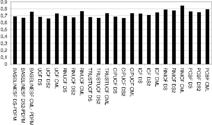
prediction accuracy mae MAE for evaluations of prediction accuracy.
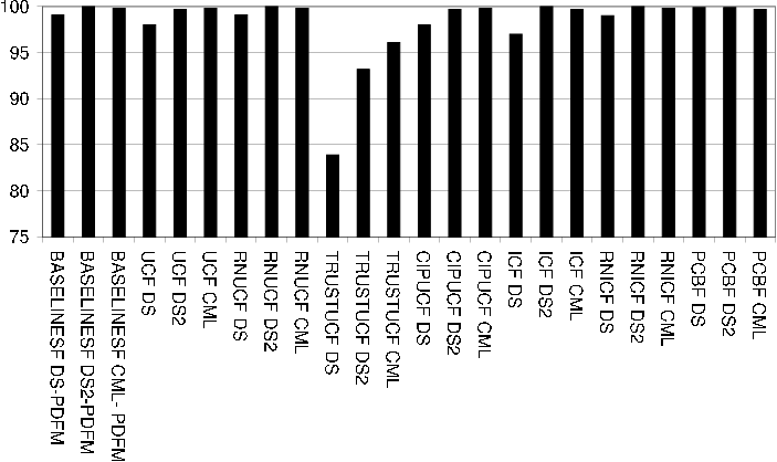
prediction accuracy coverage Coverage for evaluations of prediction accuracy.
Prediction accuracy in terms of MAE and Coverage for a select set of evaluated recommendation algorithms. Note that MAE can at most be  (in this case 4), and that Coverage is meassured in percent (%).
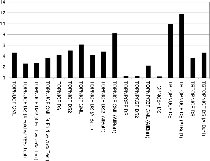
ranking relevance recall Recall for evaluations of relevance of Top-N ranking lists.
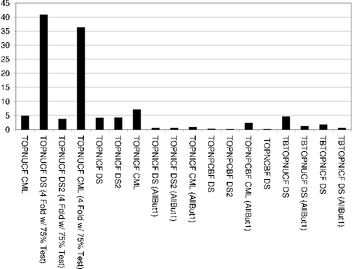
ranking relevance precision Precision for evaluations of relevance of Top-N ranking lists.
Ranking relevance in terms of Recall and Precision for all evaluated recommendation algorithms. Note that Recall and Precision is measured in percentage (%).
The following notable observations can be made on the evaluation results of the prediction accuracy.
Evaluation time Evaluations based on the DS dataset take the longest time in all cases. CML fastest.
Successful users and failed users In all cases the techniques were able to provide (almost) each user with at least one prediction. For the CML dataset Us is max all the time, for the DS and DS2 dataset there's three notable cases where users fail to get any predictions, these are UCF, TRUSTUCF and CIPUCF, with trust being the most notable one with about 30 users.
Successful predictions and failed predictions Many failed predictions for TRUSTUCF, considerably worst for DS dataset. For all other techniques number of failed predictions is negligible. In those cases you can note something, it is for the DS dataset.
Coverage Near 100% coverage in all cases except for the TRUSTUCF technique for which it is considerably lower than for the rest. Otherwise in the cases we can note anything, it is for the DS dataset the coverage is slightly lower.
Correctness Never more than 50% correctness for any technique. For baseline random has worst correctness, and PDFM highest correctness in all cases. For all other techniques, the same pattern appears, with DS2 slightly better than DS and CML.
Accuracy metrics Notable for the baseline techniques, random has clearly worst MAE, almost twice the MAE of PDFM. We can note that the RNUCF and RNICF have twice as good MAE as the random baseline. If we try out different methods of forming neighborhoods, clearly we should want to outperform the RNUCF and RNICF techniques, and not just the baseline random predictions. For all techniques independent of dataset, we get a MAE of approximately
 . For all remaining measurements of prediction accuracy (NMAE, MSE, etc.) the same pattern can be detected as for MAE. Meaning the accuracy is always best for the DS2 dataset, followed by DS and CML.
As we can see the choice of dataset has impact on the results, MAE varies (not much, but little) between the datasets, as does the coverage, therefore comparison of algorithm accuracy must be done on exactly the same datasets. All techniques, except the random ones, have more or less the same accuracy. Notable is that the baseline user mean and item mean which does not require much computing time nor memory are not far off from the best performing techniques. But using those techniques, you can not claim to produce personalized predictions. For example, the theoretically quite sound TRUSTUCF technique gives us more reason to state our predictions are personalized, but reduces coverage considerably and increases computation time. The reduction in coverage we believe has to do with the sparsity of the data, the CML dataset is least sparse, the coverage when using i.e. the TRUSTUCF technique is less noticeable (only shows a decrease in coverage of 5%) than for the DS and DS2 dataset. Choice of metric based on our evaluations does not matter much since the same characteristics can be seen independent of the metric. Therefore we agree with [herlocker00understanding] who argues that a standardized metric for evaluation of accuracy of predictions should be the MAE.
In many papers an increase in the second or third decimal of the MAE seems to be reason for claims for a significant improvement in predictive accuracy of a recommender system. Sometimes statistical tests are used to ensure that this really is a significant improvement. However, such tests do not mean that any one user of the system will notice a difference, and only has a meaning when comparing against other evaluation results and your own algorithms (e.g. will a user care whether he is predicted 4 or 4.5?).
The following notable observations can be made on the evaluation results of the ranking list relevance:
Successful and failed Users Number of failed users is heavily dependent on the size of the test data, as is to be expected and can be seen when studying e.g. the evaluation results for the TOPNUCF technique for the CML dataset when using a 10-Fold and 4-Fold (with 75% test data) evaluation data set. Since we had the requirement that we wouldn't make any predictions unless the active user had seen at least 20 of the movies similar to the active movie, the number of failed users for the TOPNICF technique was higher for the DS and DS2 dataset than for the CML dataset since the average number of ratings per user is twice as high in the CML dataset. This requirement however increases the confidence of the recommendations, and was deemed a necessary requirement to get any useable results when using the TOPNICF technique. For all other techniques where applicable no such minimum restriction is put on the neighborhood sizes, and the number of failed predictions also goes down for those techniques.
Successful and failed Top-N lists For all techniques the number of failed Top-N lists is very high. For the CML dataset the best results are obtained, with around "only" half of the Top-N lists containing no relevant items. Notable is that almost none of the Top-N lists produced by the TOPNCBF technique contain any relevant items.
Average size of Top-N ranking list Same observations as for "Successful and failed Users".
Coverage Since, as observed, there are few successful Top-N lists the coverage should be low.
Recall and precision The effect of the size of the test data when it comes to recall and precision is clearly visible when studying e.g. the evaluation results for the TOPNUCF technique for the CML dataset when using 10-Fold and 4-Fold (with 75% test data) evaluation data sets. We see that with a small test data set with few known relevant movies, recall increases but at the same time precision decreases, as is to be expected. We also see the effect of having more known relevant movies, recall is decreased but precision is increased. Since as previously observed few Top-N lists containing any relevant items are returned, the recall should be low, similarly for precision. If we look at the recall for the TOPNUCF technique for the DS and DS2 dataset we see that the recall is almost the same, but precision is 40.8% for the DS dataset and only 3.7% for the DS2 dataset. The change of dataset clearly resulted in a decreased precision. If we look at the number of Top-N lists we see that for the DS dataset there's many failed Top-N lists, i.e. lists with no relevant items, however the majority of these failed Top-N lists are also empty, this is not the case for the DS2 dataset where almost all failed Top-N lists are not empty. Since precision is the number of returned relevant items divided by the total number of returned items, the empty Top-N lists accounts for the higher precision.
F1 and Utility An interesting observation is that even though F1 and Utility are two different formulas, they produce almost identical results in all cases except when AllBut1 is used. Which is due to the fact that the F1 metric is dependent on the size of the test data, while Utility isn't.
AFHP Interesting to note is that in most cases the first known relevant item is on average encountered on the fourth place in the Top-N lists.
Overall, given our results for the ranking evaluation, none of the algorithms produce Top-N lists containing especially many items that had been assumed relevant for the user. In related studies of Top-N recommendations, such as [mclaughlin04collaborative] , [sarwar00analysis] and [karypis01evaluation] , reported precision (for similar datasets) is overall low and high recall is not reported together with high precision.
The measuring of relevance for ranking lists proves quite difficult, recall and precision is awfully low within the evaluation model applied. For the same recommendation algorithm, higher precision can be achieved when manipulating the form of the evaluation data such that the test dataset is larger, however this decreases recall. Instead the goal is to naturally to alter the algorithm to increase precision, without decreasing recall.
It is not always clear how relevance is defined in different studies, as discussed previously different definitions are possible and must be made clear. In our evaluations rated items were considered relevant and all other items were considered non-relevant. This means that for each user there is a larger number of non-relevant items which will bias the results towards low relevance.
In summary, when evaluating your recommendation algorithms, pay attention to additional accuracy measures when evaluating the prediction accuracy, look at MAE, Coverage and Correctness as well. Also give thought to low measurements, consider e.g. whether a low coverage such as 40% as opposed to a near 100% coverage is really a bad measurement, if for example the MAE goes up with 100% coverage, is it then not better to settle for 40% coverage with low MAE instead? As also suggested elsewhere [riedl05introduction] , the focus on evaluation of recommender systems, adjusting algorithms to lower MAE and other measurable quantities, should not be the only focus. Focus should be made on creating useable recommender systems with innovative, experimental and interesting ways of interacting and understanding the recommender system. This does not mean only focusing on the interface, but a focus on from the beginning selecting sensible or interesting approaches to recommendation systems where in the end the recommendation trail is what's presented to the user. As such no incorrect recommendations can be made, eliminating the need for a algorithmic evaluation, only well motivated recommendations will be made that either appeal or do not appeal to the user, but which are never strictly incorrect predictive guesses.