Chapter 4 - Self-Organizing Maps
The SOM paradigm was originally motivated by an attempt to explain some functional structures of the brain. Quite surprisingly, however, the SOM turned out to be very useful in exploratory data analysis and started to live a life of its own: some 6000 scientific articles have been based on it.
Teuvo Kohonen, WSOM 2005, 5th Workshop On Self-Organizing Maps.
One of the main features of artificial neural networks is the ability to adapt to an environment by learning in order to improve its performance to carry out whatever task its being trained for. The learning paradigm we will be working with here is the unsupervised learning paradigm and we will use it with competitive learning rules.
Unsupervised learning can also be thought of as self-organized learning [haykin94neuralnetworks] , in which the purpose is to discover significant patterns or features in the input data, and to do the discovery without a teacher. To do so, a self-organizing learning algorithm is provided with a set of rules of local nature, which enables it to learn to compute an input-output mapping with specific desirable properties (by local it is meant that the effect of changing a neurons synaptic weight is confined to its immediate neighborhood). Different structures of self-organizing system can be used. For example, feedforward networks consisting of an input layer and an output layer with lateral connections between the neurons in the output layer can be used or a multilayer feedforward network in which the self-organization proceeds on a layer-by-layer basis. Regardless of the structure, the learning process consists of repeatedly modifying the synaptic weights of all the connections in the system in response to some input, usually represented by a data vector, in accordance with the set of prescribed rules, until a final configuration develops. Of course, the key question here is how a useful configuration finally can develop from self-organization. The answer to this can be found in the following observation made by Alan Turing in 1952:
"Global order can arise from local interaction."
This observation defines the essence of self-organization in a neural network, i.e, many randomly local interactions between neighboring neurons can coalesce into states of global order and ultimately lead to coherent behaviour.
Haykin [haykin94neuralnetworks] identifies three different Self-Organizing Systems: Self-organizing systems based on Hebbian learning , systems based on competitive learning , also known as self-organizing (feature) maps and systems rooted in information theory, emphasizing the principle of maximum information preservation as a way of attaining self-organization. Only Self-Organizing systems based on competitive learning are considered in this text, i.e. SOMs.
In a SOM, the neurons are placed at the nodes of a lattice that is usually one or two dimensional (higher dimensions are possible but not as common) and in the final configuration of the map, which depends on the competitive learning process, the localized feature-sensitive neurons respond to the input patterns in a orderly fashion, as if a curvilinear coordinate system, reflecting some topological order of events in the input space, were drawn over the neural network. A SOM is therefore characterized by the formation of a topographic map of the input data vectors, in which the spatial locations (i.e. coordinates) of the neurons in the lattice correspond to intrinsic features of the input patterns , hence the name " self-organizing (feature) map ".
The SOM algorithm was developed by Teuvo Kohonen in the early 1980s [kohonen82selforganizing] in an attempt to implement a learning principle that would work reliably in practice, effectively creating globally ordered maps of various sensory features onto a layered neural network. Kohonen's work in SOMs and related earlier work of David Willshaw and Cristoph von der Malsburg [willshaw76how] and Stephen Grossberg [grossberg76adaptive] , [amari80topographic] were all inspired by the pioneering work of von der Malsburg in 1973 [vondermalsburg73selforganization] . Kohonen [kohonen90som] credits the above studies for their great theoretical importance concerning self-organizing tendencies in neural systems. However, the results of the ordering of neurons was weak, no "maps" of practical importance could be produced, ordering was either restricted to a one-dimensional case, or confined to small parcelled areas of the network. Kohonen realized that this was due to the fact that the system equations used to form the maps have to involve much stronger, idealized self-organizing effects, and that the organizing effect has to be maximized in every possible way before useful global maps could be created. After some experimenting with different architectures and system equations, a process description was found that seemed to produce globally well-organized maps [kohonen82selforganizing] . In its computationally optimized form, this process is now known as the SOM algorithm [kohonen90som] . If not explicit stated, the main reference source for the rest of this chapter is Kohonens book entitled "Self-Organizing Maps" , sometimes also referred to as [kohonen01som] .
Brain maps
The nineteenth century saw a major development in the understanding of the brain. At an overall anatomic level, a major achievement was the understanding of localization in the cerebral cortex, e.g. that the cortex of the human brain is organized according to functional areas such as speech control and analysis of sensory signals (visual, auditory, somatosensory, etc) [brain areas] . Around 1900, two major steps were taken in revealing the finer details of the brain. In Spain, pioneering work in brain theory was done by Ramón y Cajál (e.g. 1906), whose anatomical studies of many regions of the brain revealed that the particular structure of each region is to be considered as a network of neurons. In England, the physiological studies of Charles Sherrington (1906) on reflex behaviour provided the basic physiological understanding of synapses, the junction points between the neurons [arbib03handbook] .
More recent experimental studies about the finer-structure of the brain areas has revealed that, for example, some areas are ordered according to some feature dimensions of the sensory signals, like the somatosensory area, where response signals are obtained in the same topographical order on the cortex in which they were received at the sensory organs. These structures are called maps [somatotopic] . There are three types of neuronal organizations that can be called "brain maps": sets of feature-sensitive cells (single neurons or groups of neurons that respond to some distinct sensory input), ordered projections between neuronal layers and ordered maps of abstract features (feature maps that reflect the central properties of an organisms experiences and environment).These brain maps can extend over several centimetres such as, for example, the somatotopic map. Based on numerous experimental data and observations, it thus seems as if the internal representations of information in the brain are organized and spatially ordered, i.e. groups of neurons dealing with similar features are also located near each other. Although the main structure of the brain is determined genetically, there are reasons, due to its complexity and dynamically nature, that some other fundamental mechanisms are used in the creation of the brain structure. It was the possibility that the representation of knowledge in a particular category of things in general might assume the form of a feature map that is geometrically organized over the corresponding piece of the brain that made Kohonen to believe that one and the same general functional principle might be responsible for self-organization of widely different representations of information [kohonen01som] .
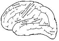
brain areas Brain areas.
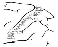
somatotopic The somatotopic map.
Images from [kohonen01som] showing the localization in the cerebral cortex and ordering in the somatosensory area of the brain.
Requirements for self-organization
The self-organizing process can be realized in any set of elements, illustrated schematically in [self organizing set] , where only a few basic operational conditions are assumed [kohonen99where] : the broadcasting of the input, selection of the winner, and adaptation of the models in the spatial neighborhood of the winner.
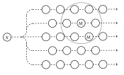
self organizing set [kohonen99where] A self-organizing set. An input message x is broadcast to a set of models mi , of which mc best matches x . All models that lie in the vicinity of mc (larger circle) improve their matching with x . Mc differs from one message to another.
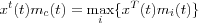
Lets consider an two-dimensional array of elements, e.g. neurons, where each element is represented by a model mi consisting of a set of numerical values (these values is usually related to some parameters of the neuronal systems such as the synaptic efficacies), and where each model will be modified according to the messages that the elements receives. First of all, assume the presence of some mechanism that makes it possible to compare the ingoing message x (a set of parallel signal values) with all models mi . In brain theory it is customary to refer to "competition" between the elements when they are stimulated by common input, and the element with the most similar model to the ingoing message is activated the most. This element is called the "winner" if it succeeds, while remaining active itself, in suppressing the activity in the neighboring elements by, for example, lateral inhibition. The winner model is denoted by mc . The above competitive process can be described as in [kohonen90som] : Competitive learning is an adaptive process, in which the neurons of the neural network are tuned to specific features of input. The response from the network then tend to become localized. The basic principle underlying competitive learning stems from mathematical statistics, namely, cluster analysis. The process of competitive learning can be described as follows:
Assume a sequence of statistical samples of a vector x = x(t) ∈ ℜn where t is time, and a set of variable reference vectors  .
.
Assume that the mi(0) have been initialized in some proper way, random selection may do.
Competitive learning then means that if x(t) can be simultaneously compared with each mi(t) at each successive instant of time then the best-matching mi(t) is to be updated to match even more closely the current x(t) .
If comparison is based on some distance measure d(x, mi) , updating must be such that if i = c is the index of the best-matching reference vector, then d(x, mc) shall be decreased, and all the other reference vectors with  left intact.
In the long run different reference vectors becomes sensitized to different domains of the input variable x . If the probability density function p(x) of the samples x is clustered, then the mi tend to describe the clusters.
The final requirement for self-organizing is then that all the models in the local vicinity of the winning model(s) also get modified such that they also will resemble the prevailing message more accurately then before. When the models in the neighborhood of the winner start simultaneously to resemble the prevailing message x more accurately, they also tend to become more similar mutually, i.e. the differences between all the models in the neighborhood of mc are smoothed. After the models mi have been exposed for different messages at different time steps all over the array, they tend to start acquire values that relate to each other smoothly over the whole array, in the same way as the original messages x in the input space do. The result is the emergence of a topographically organized map.
The Mexican Hat
The best self-organizing results are obtained if the following two partial processes are implemented in their purest forms:
Decoding of the neuron "the winner" that best match with the given input pattern.
Adaptive improvement of the match in the neighborhood of the neurons centered around the "winner"
The former operation is signified as the winner takes all function. Traditionally, the winner takes all function has been implemented in neural networks by lateral-feedback connections . For an example of a SOM algorithm that implements lateral feedback, see [sirosh93how] .
If we consider a one-dimensional lattice of neurons as depicted in [self organizing set] we see that it contains two types of connections; there are feedforward connections from an external excitation input source to the neurons in the lattice (the output layer) with associated weights and there are a set of internal feedback connections between the nodes in the lattice, both self-feedback and lateral feedback ones, also with associated weights. The magnitude and type (excitatory and inhibitory) of these weights are functions of the geometrical distance between the neurons on the lattice. Following biological motivations, a typical function that represents the values of the lateral weights versus the distance between neurons on the lattice, is the Mexican hat function. The function is proportional to the second derivative of the gaussian probability density function and is formally written as [mexican hat] , its shape is depicted in [mexican hat] .
According to the shape of the Mexican hat function, we may distinguish three distinct areas of lateral interactions between neurons [kohonen01som] as depicted in [mexican hat] .
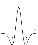
mexican hat One-dimensional "Mexican hat" function. The horizontal axis represents the distance in the lattice between neuron i and its neighbor neurons. The vertical axis represents the strength of the connections between neuron i and its surrounding neighborhood. (1) A short-range lateral excitation area. (2) A penumbra of inhibitory action. (3) An area of weaker excitation that surrounds the inhibitory penumbra; this third area is usually ignored.
By means of lateral interactions, positive(excitation) and negative(inhibition), one of the neurons becomes the "winner" with full activity, and by negative feedback it then suppresses the activity of all other cells. For different inputs the "winners" alternate.
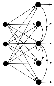
one dimensional lattice of neurons One-dimensional lattice of neurons with feedforward connections and lateral feedback connections; the latter connections are shown only for the neuron at the center of the array. First column of neurons make up the input layer, second column of neurons make up the output layer.
Hence, in presence of lateral feedback, the dynamic behavior of the network activity can be described as follows [haykin94neuralnetworks] :
Let  denote the input signals (excitations) applied to the network, where p is the number of nodes in the input layer [one dimensional lattice of neurons] .
Let Nj define the region over which lateral interactions are active, usually referred to as the neighborhood of neuron i and let cik denote the lateral feedback weights connected to neuron i inside this neighborhood.
Let  denote the output signals of the network, where N is the number of neurons in the network.
The output signal (response) of neuron i is then equal to:
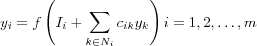
where f is a standard sigmoid-type nonlinear function that limits the value of yi and ensures that yi = 0 .
The total external control exerted on neuron j by the weighted effect of the input signals is described by:

The solution to the nonlinear equation [output signal] is found iteratively:
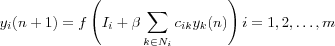
where n denotes an iteration step. The parameter  controls the rate of convergence of the iteration process.
[output signal iterative solution] represents a feedback system. The system includes both positive and negative feedback, corresponding to the excitatory and inhibitory parts of the Mexican hat function, respectively. The limiting action of the nonlinear activation function f causes the spatial response yj(n) to stabilize in a certain fashion, dependent on the value assigned to  . If
. If  is large enough, then in the final state corresponding to
  , the values of yj tend to concentrate inside a spatially bounded cluster, referred as a "activity bubble". The bubble is centred at a point where the initial response yj(0) due to the external input Ij is maximum. The width of the bubble is governed by the ratio of the excitatory to inhibitory lateral connections: the bubble becomes wider for more positive feedback, and sharper for more negative feedback. If the negative feedback is too strong, formation of the activity bubble is prevented. Consequence of bubble formations is the topological ordering among the output neurons.
However, the SOM algorithm proposed by Kohonen [kohonen90som] uses a "shortcut" or a "engineering solution" to the model described above. He suggested that the effect accomplished by lateral feedback, i.e.the bubble formation, can be enforced directly by defining a neighborhood set Nc around the winning neuron c . The lateral connections and its weights are discarded and a topological neighborhood of active neurons that corresponds to the activity bubble is introduced instead. Further, for each input signal, all the neurons within Nc are updated, whereas neurons outside Nc are left intact . By adjusting the size of the neighborhood set Nc , lateral connections can be emulated, making it larger corresponds to enhanced positive feedback, while enhancement of negative feedback is obtained by making it smaller.
The computational gain with this model is that instead of recursively computing the activity of each neuron according to [output signal iterative solution] , this model finds the winning neuron and assumes that the other neurons are also active if they belong to the neighborhood of the winning neuron. Another problem with the former model, is that the trained map can exhibit several regions of activity instead of just one. This is an immediate consequence of the Mexican hat function for lateral interactions which primarily influence neurons nearby, thus far away regions of activity has little interaction.
The SOM paradigm
With this short introduction we want to emphasize that the SOM and the SOM algorithm refers to two different aspects of the SOM paradigm, something that's not always made clear in the literature. The SOM is the result of the converged SOM algorithm.
The basic SOM is as a nonlinear, ordered, smooth mapping of high-dimensional data manifolds onto the elements of a regular, low-dimensional array. The mapping is implemented in the following way:
Define the set of input variables xj as a real vector
![x = [x_1, x_2, \dots, x_n]^T \in \Re^n](image/math91.png) .
.Associate with each element in the SOM array a parametric real vector
![m_i = [w_{i1}, w_{i2}, \dots, w_{in}]^T \in \Re^n](image/math92.png) called a model .
called a model .Define a distance measure between x and mi denoted d(x, mi) .
The image of an input vector x on the SOM array is then defined as the array element mc that best matches with x , i.e. that has the index 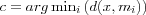 .
.
The main task is to define the mi in such a way that the mapping is ordered and descriptive of the distribution of x . The process in which such mappings are formed is defined by the SOM algorithm. This process is then likely to produce asymptotically converged values for the models mi , the collection of which will approximate the distribution of the input samples x(t) , even in an ordered fashion..
Note : It is not necessary for the models mi to be vectorial variables. It will suffer if the distance measure d(x, mi) is defined over all occurring x items and a sufficiently large set of models mi . For example the x(t) and mi may be vectors, strings of symbols, or even more general items.
The incremental SOM algorithm
Kohonen's original SOM algorithm can be seen to define a special recursive regression process, in which only a subset of the models are processed at every step. The SOM algorithm we are about to describe finds a mapping from the input data space Rn onto a two-dimensional array of nodes, called a lattice , as depicted in [som activation] .
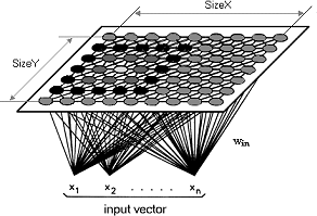
som activation A SOM of size  in which the activation area of the BMN are depicted.
With every node i , a parametric model vector , also called reference vector ![m_i = [w_{i1},w_{i2}, \dots, w_{in}]^T \in \Re^n](image/math95.png) is associated. Before recursive processing, the mi must be initialized . Random values for the components of mi may do, but if the initial values of the mi are selected with care, the convergence can be made to converge much faster. The lattice type of the array can be defined to be rectangular , hexagonal or even irregular . For visual display, hexagonal is effective.
is associated. Before recursive processing, the mi must be initialized . Random values for the components of mi may do, but if the initial values of the mi are selected with care, the convergence can be made to converge much faster. The lattice type of the array can be defined to be rectangular , hexagonal or even irregular . For visual display, hexagonal is effective.
Let ![x = [x_1, x_2, \dots, x_n]^T \in \Re^n](image/math96.png) be the input vector that is connected to all neurons in parallel via variable scalar weights wij and x ∈ ℜn be a stochastic data vector.
be the input vector that is connected to all neurons in parallel via variable scalar weights wij and x ∈ ℜn be a stochastic data vector.
The SOM can then be said to be a "nonlinear projection" of the probability density function p(x) of the high-dimensional input data vector x onto the two-dimensional array. The central result in self-organization is that if the input patterns have a well-defined probability density function p(x) , then the weight vectors associated with the models mi should try to imitate it [kohonen90som] .
Selection of the best matching node ("Winner-takes-all")
Vector x may be compared with all the mi in any metric; in many practical applications, the smallest of the Euclidian distance  can be made to define the best matching node (BMN), signified by the subscript c :

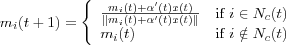
Adaptation (Updating of the weight vectors)
During learning , or the process in which the "nonlinear projection" is formed, those nodes that are topographically close in the array up to a certain geometric distance will activate each other to learn something from the same input x , see [self organizing set] . This will result in a local relaxation or smoothing effect on the weight vectors of neurons in this neighborhood, which in continued learning leads to global ordering .
This is achieved by defining a neighborhood set Nc around node c and at each learning step only update those nodes that are within Nc and keep the rest of the nodes intact. The width or radius defining which nodes are in Nc (refered to as the "radius of Nc ") can be time-variable. Experimental results have shown that best global ordering is achieved if Nc is very wide in the beginning of the learning process and shrinks monotonically with time. Explanations for this is that in the beginning a rough ordering among the mi values are made, and after narrowing the Nc , the spatial resolution of the map is improved.
The following updating process is then used:
![m_i(t + 1) =
\left\{
\begin{array}{ll}
m_i + \alpha(t)[x(t) - m_i] & \mbox{ if } i \in N_c(t)\\
m_i & \mbox{ if } i \notin N_c(t)\\
\end{array}
\right.](image/equation68.png)
where  (is the discrete-time coordinate (an integer) and
  is a scalar-valued learning-rate factor
  that decreases with time.
However, instead of using the simple neighborhood set where each node in the set is affected equally much we can introduce a scalar "kernel" function hci = hci(t) as a neighborhood function defined over the lattice nodes, then the updating process may read as:
![m_i(t+1) = m_i(t) + h_{ci}(t)[x(t) - m_i(t)]](image/equation69.png)
For convergence it is necessary that  when
when  . Usually hci(t) is a function of the distance between nodes c and i in the array, i.e.
 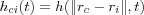 , where rc and ri denotes the coordinates of node c and i respectively in the array. With increasing
  we then have that
  .
.
Two simple choices for hci(t) occur frequently, whereas the simpler of them is the above neighborhood set Nc defined as a function of time Nc = Nc(t) , whereby  if i ∈ Nc and hci(t) = 0 if i ∈ Nc . Both
  and the radius of Nc(t) usually decreases monotonically in time.
The other choice is a much smoother neighborhood kernel, known as the Gaussian function :
where  is another scalar-valued learning-rate factor and the parameter
  defines the width of the kernel, the latter corresponds to the radius of Nc(t) above. Both
  and
and  are some monotonically decreasing functions of time.
Selection of parameters
The learning process involved in the computation of a feature map is stochastic in nature, which means that the accuracy of the map depends on the number of iterations of the SOM algorithm. We have seen that there are many parameters involved in defining and training a SOM, different values will have different effects on the final SOM. The values of the parameters are usually determined by a process of trial and error. However, the following advices based on our experience and observations made by others can provide a useful guide.
The Size of SOM determines the degree of generalization that will be produced by the SOM algorithm - the more nodes, the finer the representation of details, while the fewer nodes, the broader level of generalization. However, the same broad patterns are revealed at each level of generalization. Another issue regarding the size of the SOM, is that more nodes means longer training time. For example, a  SOM takes four times longer to train then a
  SOM. Sammon's mapping [sammon69nonlinear] can be used on the data set to get some hints on the structure of the data set and by that helping in the process of selecting number of nodes in the lattice.
The learning steps must be reasonably large, since the learning is a stochastic process. A "rule of thumb" is that for good statistical accuracy, the number of steps must be at least 500 times the number of network nodes.
The Learning rate parameter α should start with a value close to 1 and then during the first 1000 steps it should be decreasing monotonically but kept above 0.1 . The exact form of variation of  is not critical, it can be linear, exponential or inversely proportional to t . For instance,
 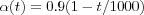 may be a reasonable choice. It is during the initial phase of the algorithm that the topological ordering of the mi occurs. This phase of the learning process is therefore called the ordering phase . The remaining (relatively long) iterations of the algorithm are needed for the fine adjustment of the map; this second phase of the learning process is called the convergence phase . For good statistical accuracy,
  should be maintained during the convergence phase at a small value (on the order of 0.01 or less) for a fairly long period of time, which is typically thousands of iterations. Neither is it crucial whether the law for
  decreases linearly or exponentially during the convergence phase.
The Neighborhood function can be chosen to be the simple neighborhood-set definition of hci(t) if the lattice is not very large, e.g. a few hundred nodes. For larger lattices, the Gaussian function may do.
The size of the Neighborhood must be chosen wide enough at the start so the map can be ordered globally. If the neighborhood is too small to start with, various kinds of mosaic-like parcellations of the map are seen, between which the ordering direction changes discontinuously. This phenomena can be avoided by starting with a fairly wide neighborhood set Nc = Nc(0) and letting it shrink with time. The initial radius can even be more than half the diameter of the network. During the first 1000 steps or so, when the ordering phase takes place, and  is fairly large, the radius of Nc can shrink linearly to about one unit, during the convergence phase Nc can still contain the nearest neighbors of node c .
Incomplete data
The SOM algorithm is very robust, compared to other neural networks. One problem that frequently occurs in practical applications, especially in applying methods of statistics, is caused by missing data. It has been shown that the SOM algorithm is very robust to missing data in [samand92selforganization] , in fact, they claimed that it is better to use incomplete data then to simply discard the dimension from which there are missing data. However, if a majority of the data is missing from a dimension, its better to discard that dimension totally from the learning process [kaski97thesis] . In training of the SOM with incomplete data, the contribution of missing data is assumed to be zero, i.e.  . Note that the reference vector is represented in every dimension and only those dimension that are represented by the input vector causes changes in the reference vector.
Quality measure of the SOM
Although some optimal map always exists for the input data, choosing the right parameters from start is a tricky task. Since different parameters and initializations gives rise to different maps, it is important to know whether the map has properly adapted itself to the training data. This is usually done with an cost function that explicitly defines the optimal solution but since it has been shown that the SOM algorithms not the gradient of any cost function, at least in the general case, other quality measures has to be used. Two commonly used quality measures that can be used to determine the quality of the map and helping in choosing suitable learning parameters and map sizes are the average quantization error and the topographic error.
Average quantization error
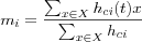
Average quantization error is as a measure of how good the map can fit the input data and the best map is expected to yield the smallest average quantization error between the BMNs mc and the input vectors x . The mean of  , defined via inputting the training data once again after learning, is used to calculate the error with the following formula:
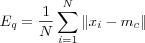
where N is the number of input vectors used to train the map
A SOM with a lower average error is more accurate than a SOM with higher average error.
Topographic error
Topographic error measures how well the topology is preserved by the map. Unlike the average quantization error, it considers the structure of the map. For each input vector, the distance of the BMN and the second BMN on the map is considered; if the nodes are not neighbors, then the topology is not preserved This error is computed with the following method:
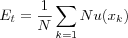
where N is the number of input vectors used to train the map and u(xk) is 1 if the first and second BMN of xk are not direct neighbors of each other. Otherwise u(xk) is 0.
Note : In measuring the quality of a SOM consideration must be taking for both the average expected error as well as the topographic errors.
Summary of the SOM algorithm
The essence of Kohonen's SOM algorithm is the idea of discarding the Mexican hat lateral interactions for a time depended "topological neighborhood" function as a way of algorithmically emulate the way self-organizing takes place in biological system. The algorithm can be summarized in two steps:
Locate the BMN
Increase matching at this node and its topological neighbors
The two steps are however usually carried out as follows:
- 1. Initialize network
For each node i , initialize corresponding reference vector mi at random. Set the initial learning rate a close to unity and the radius s to be at least half the diameter of the lattice.
- 2. Present input
Present the input vector x(t) at time t to all nodes in the lattice simultaneously.
- 3. Similarity matching
Find the BMN c at time t using the minimum-distance Euclidian criterion:

where N is the total number of nodes in the lattice.
- 4. Update
Adjust the reference vector mc and all reference vectors mi within the neighborhood of the winning node c using:
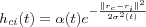
![m_i(t+1) = m_i(t) + h_{ci}(t)[x(t)-m_i(t)] \mbox{ where } h_{ci}(t) = \alpha(t)e^{- \frac{\|r_c - r_i\|^2}{2\sigma^2(t)}}](image/equation74.png)
- 5. Repeat
Decrease learning rate and the width of the neighborhood. Repeat from step 2 by choosing a new input vector
 until a predefined stop criteria is reach.
The Dot-Product SOM algorithm
Normalization is not necessary in principle, but sometimes it may be necessary to normalize the input x before it is used in the algorithm. Reasons for this can be to ensure that the resulting reference vectors are kept in the same dynamic range. Another aspect is that it is possible to apply many different metrics in matching, however then the matching and updating laws should be mutually compatible with respect to the same metric. For instance, if the dot-product definition of similarity of x and mi is applied, the learning equations should read:
where  , for instance,
  . This process automatically normalizes the reference vectors at each step. Normalization usually slows down training process but during matching, the dot-product criterion is very simple and fast. The Euclidian distance and the dot products are the most widely used matching criteria's, although many others have been used.
The batch SOM algorithm
Another type of SOM algorithm is the batch(-map) SOM algorithm [kohonen93things] , it is also an iterative algorithm, but instead of using a single data vector at time t , the whole data set is presented to the map before any adjustments are made -- hence the name "batch". The algorithm is outlined below:
- Selection of the BMN
Consider a set of input samples X and a two-dimensional lattice where with each node i a reference vector mi is associated. The initial values of the mi can be selected at random from the domain of input samples. With the use of a distance measure d(x, mi) , the node that is most similar to the input x ∈ X is found and x is then copied into a sublist associated with that node.
- Adaptation (Updating of the reference vectors)
After all input samples x ∈ X have been distributed among the nodes sublists, the reference vectors can be updated. This is done by finding the "middlemost" samples
 or
or  for each node i and replacing the old value of mi with
  or
or  .
.Start by considering the neighborhood set Ni around reference vector mi . The neighborhood set consists of all nodes within a certain radius from node i . In the union of all sublists in Ni , find the "middlemost" sample
 which have the smallest sum of distances from all the samples x(t) where t ∈ Ni . This "middlemost" sample can be either of two types:
Generalized set median: If the sample
 is part of the input samples x ∈ X .
Generalized median: If the sample
 is not part of the input samples x ∈ X . Since we are only using a sample of inputs x ∈ X it may be possible to find an item
  that has an even smaller sum of distances from any of the x ∈ Ni , this item
  is called the generalized median.
The middlemost sample
 or
or  that has been found is used to replace the old value of mi . This is done for each node i , by always considering the neighborhood set Ni around each node i , i.e. by replacing each old value of mi by
  or
or  in a simultaneous operation.
The above should then be iterated, i.e. all the samples x ∈ X are again distributed into the sublists (which will now most likely change since each mi has been updated in the previous iteration) and new medians are computed.
Formally, the above process uses a concept known as Voroni tessellation when forming the neighborhood sets. It is a way of partitioning a set of data vectors into regions, bordered by lines, such that each partition contains a reference vector mi that is the "nearest neighbor" to any vector x within the same partition. These lines together constitute the Voronoi tessellation. All vectors that have a particular reference vector as their closest neighbor are said to constitute a Voronoi set V . That is, the reference vectors mi and the search for the BMN defines a tessellation of the input space into a set of Voronoi sets Vi , defined as:

In each training step, the map units are associated with one such Voronoi set, i.e. the sublist of each reference vector mi continaing the data vectors x that have it as BMN constitute a Voronoi set.
If a general neighborhood function hci is also used, then the the formula for updating the reference vectors becomes:
where c is the bmn for the current sample x .
This algorithm is particularly effective if the initial values of the reference vectors are roughly ordered. This algorithm contains no learning rate parameter and therefore it seems to yield more stable asymptotic values for the mi compared to the original SOM algorithm [kohonen93things] .
The SOM as a clustering and projection algorithm
The SOM is very useful in producing simplified descriptions and summaries of large datasets. It creates a set of topographic ordered reference vectors that represents the data set on a two-dimensional grid. This process can be described in terms of vector quantization (VQ) and vector projection (VP). The combination of these two methods is called vector quantization-projection (VQ-P) methods [vesanto99sombased] , and clearly, the SOM can be categorized as such.
VQ is used as a way of reducing the original data to a smaller but still representative set of the original data. In the SOM, the reference vectors for the models or nodes in the grid, are representative for a larger set of data vectors in the input space.
VP is used to project high-dimensional data vectors as points on a low-dimensional, usually 2D, display. In the SOM, this is defined as the location of the data vectors' BMN.
In the SOM process, VQ and VP interacts with each other, in contrast to a serial combination of the two methods, where VQ is performed first (by a clustering algorithm like K-means ) and then a VP is performed (by a projection method like Sammons's mapping ).
Vector quantization
Clustering means partitioning of a data set into a set of clusters Ki ,  , where each cluster is supposed to contain data that is highly similar. One definition of optimal clustering is a partitioning that minimizes distances within and maximizes distance between clusters where distance is used as a measure of dissimilarity , i.e. the magnitude of the distance implies how "unlike" two data items are. The Euclidian distance is a commonly used distance criterion. A survey of different clustering algorithms can be found in [jain99data] .
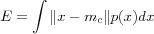
Algorithms based on VQ performs an elementary unsupervised clustering and classification of the data vectors in an (input) space [kohonen01som] . Formally the goal of VQ can be stated as; given a set of input data vectors x ∈ ℜn find a finite number of reference vectors  that form a quantized approximation of the distribution of the input data vectors. Once suitable reference vectors have been determined (using a VQ algorithm), VQ (or approxomation) of an input vector x simply means finding the reference vector mc closest to the input vector x (in input space). Finding the closest reference vector is usually done using the Euclidian metric as in
 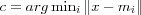 where c is the index of the closest reference vector mc . The optimal formation of reference vectors, when using the Euclidean metric, means finding reference vectors that minimize the average expected square of the quantization error , defined as:
where p(x) is a probability density function of x for the input space and the integration is performed over the entire input space. Since a closed form (*) solution for the determination of the mi is not available, at least for a general p(x) , an iterative approximation algorithm is used. See [kohonen01som] for the derivation of such an algorithm and a more rigorous study of VQ. The SOM is therefore very closely related to VQ-based clustering algorithms.
Competetive (or winner-takes-all) neural networks can be used to cluster data. Kohonen has developed two methods for automatic clustering of data, one supervised methods called learning vector quantization and one unsupervised methods called the SOM. Both methods build on the VQ methods originally developed in signal analyis for compressing (signal) data. In learning vector quantization only one or two winning node's reference vectors are updated during each adaptation stage, whereas in the SOM the reference vectors for a neighborhood of nodes in the SOM's lattice are updated simultaneously.
One well known clustering algorithm that performs clustering in a similar way as VQ is the well known K-means algorithm . The K-means algorithm is a very popular clustering algorithm, mainly because it is easy to implement and its time complexity is O(n) , where n is the number of data vectors. The algorithm is sensitive to the choice of initial reference vectors and may therefore converge to a local minima. The objective of the K-means algorithm is to minimize the distance between the input data vectors and the reference vectors. The algorithm minimizes the sum of squared errors:
where c is the number of clusters and the reference vector mi is the mean of all vectors x in the cluster Ki .
The K-means algorithm first selects K data vectors, from the set of data vectors to cluster, to be used as initial reference vectors mi . Next K clusters are formed by assigning each available data vector x to its closest reference vector mi . The mean  for each cluster is the computed and used as the new value of mi . The process is repeated until it is determined that the objective function has reached a minima, i.e. there's a minimal decrease in the sum of squared errors. Note that we have explained the K-means algorithm in SOM terminology, usually the reference vectors is defined in terms of a centroid, which is the mean of a group of points.
The K-means algorithms and the SOM algorithms are very closely related, if the width of the neighborhood function is zero (including only the BMN) then the incremental SOM algorithm acts just as the incremental K-means algorithm. Similarly, the batch version of the K-means algorithm is closely related to the batch SOM algorithm. Although they are very closely related, in K-means the K reference vectors should be chosen according to the expected numbers of clusters in the data set, whereas in the SOM the number of reference vectors can be chosen to be much larger, irrespective of the number of clusters [kaski97thesis] .
Vector projection
The purpose of projection methods is to reduce the dimensionality of high dimensional data vectors. The projection represents data in a low dimensional space, usually two-dimensional, such that certain features of the data is preserved as good as possible [kohonen01som] . Typically, such features are the pair wise distances between data samples or at least their order and subsequently preservation of the shape of the set of data samples. Projection can also be used for the visualization of data if the output space is at most 3 dimensional.
Several projection methods are discussed in [kaski97thesis] , linear projections such as principal component analysis (PCA), nonlinear projections such as multidimensional scaling (MDS) methods and the closely related Sammon's mapping . Kohonen [kohonen01som] also mentions nonlinear PCA and curvlinear component analysis (CCA). However, these methods seem to only differ in how the different distances are weighted and how the representations are optimized [kaski97thesis] .
Linear projection
PCA was first introduced by Pearson in 1901 and further developed by the statistician Hotelling in 1933 and then later by Loève in 1963 and is a widely used projection method. PCA can be used to display the data as a linear projection on a subspace of lower dimension of the original data space that best preserves the variance in the data but since PCA describes the data in terms of a linear subspace, it cannot take into account nonlinear structures, structures consisting of arbitrarily shaped clusters or curved manifolds [kaski97thesis] . Assuming that the dataset is represented in a proper way as data vectors, PCA is done by the use of matrix-algebra(*) : first the covariance matrix of the input data is calculated and then, secondly, the eigenvectors and eigenvalues are calculated for this matrix. The principal components of the data set is then the eigenvector with the highest eigenvalue. In general, the eigenvectors are ordered by their eigenvalues, from high to low. By leaving out eigenvectors with low eigenvalues, the final dataset will be of lesser dimension than the original one. Of course, some information may be lost, but since the eigenvalues were low, the loss will be minor. It should be noted that there exists a nonlinear version of PCA, called principal curves . However, as it turns out, to be used in practical computations, the curves have to be discretizated and discretizated principal curves are then essentially equivalent to the SOMs [kohonen01som] . Thus, the conception of principal curves is only useful in providing one possible viewpoint to the properties of the SOM algorithm.
Non-linear projection
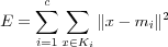
In 1969, a projection method called, Sammon's mapping , was developed [sammon69nonlinear] . Sammon's mapping is closely related to the group of metric based MDS methods in which the main idea is to find a mapping such that the distances between data vectors in the lower dimensional space is as similar as possible to the distance of the corresponding data vectors in the original metric space [kohonen01som] . The basic idea in Sammon's mapping and other projection methods is to represent each high-dimensional data vector as a point in a 2 dimensional space and then arrange these points in such a way that the distances between the points resemble the distances in the original space (defined by some metric) as faithfully as possible. More formally, assume we are given a distance matrix M consisting of pair wise distances between all vectors xi and xj in the input space ℜn , where n is the dimensionality of the input space. M is then defined by its elements dij , where  . Further, let ri ∈ ℜ2 be the location or coordinate vector of the data vector xi ∈ ℜn . With N we denote the distance matrix consisting of the pair wise distances between all the coordinate vectors ri and rj in the 2 dimensional space ℜ2 measured with the Euclidian norm
  . The goal is then to adjust the ri and the rj vectors on the ℜ2 plane so that the distance matrix N resembles the distance matrix M as well as possible, i.e. to minimize a cost function represented as an error function E by way of a iterative process. The error E function is defined as (following the notation used in [kohonen01som] :
This leads to a configuration of the ri points such that the clustering properties of the xi data vectors are visually discernible from this configuration. Thus, the inherent structure of the original data can be told from the structure detected in the 2-dimensional visualization. If we compare the above methods with each other, we see that the difference lies in how the distances are weighted. In Sammon's mapping small distances in input space are weighted as more important, in CCA the small distances in output space are weighted as more important and in the case of MDS no weighting is used resulting in larger distances having more impact on the error function. The weighting of distances results in projections that better preserve the local shape of the structure of the input space, whereas no weighting as in the MDS case gives a better global shape of the structure in the input space.
Kohonen recommends that Sammon's mapping is used for a preliminary analysis of the data set used for SOMs, because it can roughly visualize class distributions, especially the degree of their overlap.
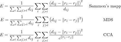
In [Figures pca projection , sammon projection , som projection ] projections based on the same dataset are shown, the dataset is a rating dataset involving 17 movies and 808 users. Comparing [pca projection] with [sammon projection] shows that Sammon's mapping spreads the data in a more illustrative way then PCA. In [som projection] the effect of using a fixed grid size combined with the topographic ordering that is enforced by the SOM algorithm is shown.
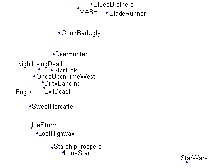
pca projection Linear projection of the data as points onto the two-dimensional linear subspace obtained with PCA.
sammon projection Non-linear projection onto a two dimensional space using Sammons's mapping.
som projection Data placed on their BMN in a 10x10 grid using a SOM obtain using the incremental SOM algorithm.
projections Projections using different projection algorithms of the same 808-dimensional dataset consisting of ratings on 17 movies by 808 users.
Comparison of the SOM to other VQ and VP algorithms
The SOM as discussed by Kohonen in [kohonen01som] combines clustering and visualization operations, however, some essential differences to the methods previously described can be found in [kohonen01som] and [kaski97thesis] :
The SOM represents a open set of multivariate data vectors by a finite set of reference vectors mi ,like in K-means clustering. This is not the case in the above discussed projection methods where the number of input samples equal the number of outputs.
Unlike K-means, the number of reference vectors should not equal the number of expected clusters, instead there numbers of reference vectors should be fairly large. This has to do with the neighborhood function, which makes neighboring nodes on the grid more similar each other, and thus neighboring nodes reflect the properties of the same rather than different clusters. The transition from one cluster to another on the grid is gradual taking place over several nodes. If the goal is to create a few, but quantitative clusters, the SOM has to be clustered. [vesanto00clustering]
The SOM represents data vectors in a orderly fashion on a (usually) two-dimensional regular grid and the reference vectors are associated with the nodes of the grid. That is, the SOM tries to preserve the topology instead of the distance between data samples, whereas, for example, Sammon's mapping tries to preserve the metric with an emphasize for preserving the local distance between data samples. The grid structure also discretizate the output space, whereas Sammon's mapping has continuous outputs.
It is not necessary to recompute the SOM for every new samples, because if the statistics can be assumed stationary, the new sample can be mapped onto the closest old reference vector. In Sammon's mapping, for example, the mapping of all data samples is computed in an simultaneous optimization process, meaning that, with new data samples a new optimal solution exists. Therefore, no explicit mapping function is created since the projection must be recomputed for every new data sample.
Sammon's mapping can very easy converge to a local optimal solution, so in practice, the projection most be recomputed several times with different initial configurations. The SOM algorithm is found to be more robust to this if learning is started with a wide neighborhood function that gradually decreases to its final form.
Different methods, like the SOM, K-means and various projection methods, all display properties of the data set in slightly different ways, therefore, a useful approach could be to combine several of them. In the paper [flexer97limitations] , K-means and Sammon's projection is combined into a serial VQ-P method and compared against the SOM. They report that their combined method outperforms the SOM as a clustering and projection tool. However, it seems like their performance measure favors distance preserving algorithms and the SOM is not intended for distance preserving, instead the SOM orders the reference vectors on a lattice structure in such a way that local neighborhood sets in the projection are preserved. In a study done by [venna01neighborhood] a new concept is defined: the trustworthiness of the projection, meaning that if two data samples is closed to each other in output space, then they are more likely to be near each other in the input space. The SOM is compared to other methods like the PCA, non-metric MDS and Sammon's mapping and are found to be especially good at this. It is also shown that the SOM is good at preserving the original neighborhood set in the projection. Although PCA and non-metric MDS is found to be better on this. For discrete data, neighborhoods of data vectors is defined as sets consisting of the k closest data vectors, for relatively small k .
Visualizing the SOM
Different kinds of methods for visualizing data using the SOM and other VQ-P methods are discussed in the paper [vesanto99sombased] . Three goals of visualization is defined; to get an idea of the structure and the shape of the data set, for example, if there is any clusters and outliers. Secondly, analysis of the reference vectors in a greater detail, and third, examining new data with the map, i.e. the response from the map has to be quantified and visualized.
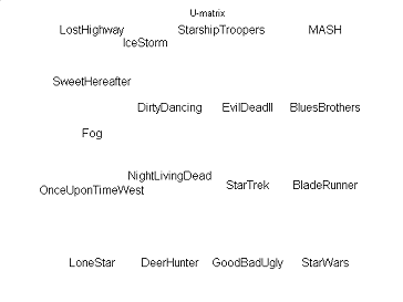
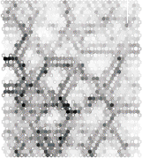
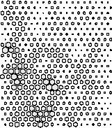
As for the first goal, while projections give a rough idea of clusters in the data, to actually visualize the clusters on the SOM, techniques based on distance matrices is commonly used. The distance matrix can contain all distances between the nodes reference vectors in the lattice as well as their immediate neighbors, like in the Unified distance matrix (U-matrix), as illustrated in [som visualization umatrix] or just a single value for each node, representing either the minimum, maximum or average distance for the nodes to its neighbors, as illustrated in [som visualization distance matrix] . A related technique is to use colors, i.e, same color is assigned to nodes that are similar, as illustrated in [som visualization similarity coloring] .
som visualization umatrix U-Matrix
som visualization distance matrix Distance Matrix
som visualization similarity coloring Similarity Coloring
som visualization The U-matrix som visualization umatrix is a graphic display frequently used to illustrate the clustering of the reference vectors in the SOM, it represents the map as a regular grid of nodes where the distance between adjacent node's reference vectors is calculated and presented with a coloring scheme. A light coloring between nodes signifies that the reference vectors are close to each other in the input space and A dark coloring between the nodes corresponds to large distances and thus a gap between the reference vectors in the input space. Dark areas can be thought of as clusters separators and light areas as clusters. This is helpful when one tries to find clusters in the input data without having information if there is any. som visualization distance matrix In the Distance Matrix each map node is proportional to the average distance to its neighbors. som visualization similarity coloring In the Similarity Coloring map nodes that are similar have the same color.
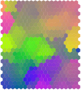
The U-matrix can bee seen as several component planes stacked on top of each other. Each component plane shows the values of a single vector component in all nodes of the map, hence, together they can be seen as constituting the whole U-matrix. Component planes are commonly used in the analysis of reference vectors since they can give information such as the spread of the values of a component or they can also be used in correlation hunting, i.e. finding to component planes with similar patterns [component planes] .
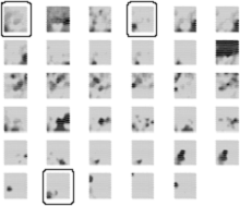
component planes Component planes, useful for correlation hunting.
In the examination of new data, the response from the map can be as simple as just pointing out the BMN for that data. Histograms can be used for multiple vectors. Often some form of accuracy is also measured to give some information whether the sample is close to the mapped BMN or very far.
Properties of the SOM
Once the SOM algorithm has converged, the SOM computed by the algorithm displays important statistical characteristics of the input data. The SOM can be seen as a nonlinear transformation φ that maps the spatially continuous input space X onto the spatially discrete output space L , as depicted in [som] [haykin94neuralnetworks] . This transformation, written as  can be viewed as an abstraction of [bmn] , finding of the BMN. The topology of the input and output space are defined respectively by the metric relationship of vectors x ∈ X and the arrangement of a set of nodes of a regular two-dimensional grid. If we consider this in a neurobiological context, the input space X may represent the coordinate set of somatosensory receptors distributed densely over the entire body surface, then output space L will represent the set of neurons located in the layer of the cortex which the somatosensory receptors are confined.
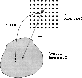
som [haykin94neuralnetworks] Illustration of a relationship between the SOM φ and a reference vector mc of a BMN c . Given an input vector x, the SOM φ identifies a BMN c in the output space L . The reference vector mc for node c can then be viewed as a pointer for that node into the input space X .
Approximation of the input space
The SOM φ , represented by the set of reference vectors  in the output space L , provides an approximation to the input space X .
This property comes from the fact that the SOM performs VQ, as discussed earlier, where the key idea is to use a relatively small number of reference vectors to approximate the original vectors in input space.
Topological ordering
The SOM φ computed by the SOM algorithm is topologically locally and globally ordered in the sense that nodes that are close to each other on the grid represents similar data in the input space.
That is, when data samples are mapped to those nodes on the lattice that have the closest reference vectors, nearby nodes will have similar data samples mapped onto them.
This property is a direct consequence of the updating process [neighborhood function] . It forces the reference vector mi of the BMN c to move toward the input vector x , and when used with a wide neighborhood kernel in the beginning of the learning process that slowly decreases during training, a global ordering is guaranteed (since it has the effect of moving the reference vectors mi of the closest nodes(s) i along with the BMN c ).
Illustration of the ordering principle implemented by the SOM
The difference between a locally and globally ordered SOM φ on one hand and a SOM φ that is only locally ordered can be illustrated if we think of the SOM φ as an elastic net that is placed in input space. (Such an illustration however requiers a special case, such as when both the input and output space is two dimensional. Keep in mind that the input space is usually of a very high dimension and that ordering is not well defined in higher dimensions, it is however useful to imagine something similar occuring in higher dimensional cases.)
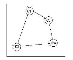
For a two-dimensional input space with the point distribution as shown in [input space] , four distinct clusters can easily be detected by visual inspection, these are denoted in the figure by  and c4 .
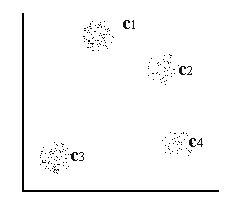
input space Two-dimensional input space consisting of four distinct clusters denoted  and c4 .
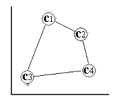
The output space consists of a regular two-dimensional grid structure of four nodes, where the corresponding reference vector corresponds to some coordinates in input space X [output space] .
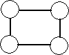
output space Two-dimensional grid structure with four nodes (output space).
The goal of the SOM algorithm is to find suitable coordinates for the reference vectors such that the collection of grid nodes follows (or approximates) the distribution of the data points in input space in such a way that neighboring nodes are more alike than nodes farther apart. Two nodes are said to be similar if they represent similar data points in input space. If this is true, then a grid is said to be globally and locally ordered and is referred to as an topologically ordered SOM φ . In order to illustrate this property of the SOM φ , we will look at a SOM φ that is locally ordered only and one that is both locally and globally ordered.
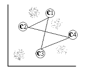
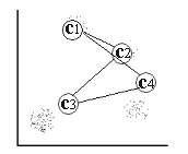
In the first case, the SOM has been trained with a neighborhood size of zero, i.e. only the BMN is updated for every data point, resulting in the grid depicted in [locally ordered som] . In the second case, the SOM has been trained with a neighborhood function that monotonically decreasing over time, i.e. more nodes are affected by the same data points in the beginning of the training than in the end of the training of the SOM. The resulting grid is depicted in [globally ordered som] . Each node is labelled with the cluster in input space that it represents.
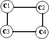
locally ordered som A locally ordered SOM~ φ .
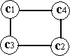
globally ordered som A locally and globally ordered SOM φ .
ordered som SOM with nodes labeled with the cluster in input space they represent.
As can be seen in [locally ordered som] and [globally ordered som] , the nodes represent different clusters and the effect of this can be detected if the labeled nodes in the figures are placed in input space while keeping their connections between each other. This "stretch" effect of the SOM φ illustrates clearly the ordering property of the SOM psi , nearby nodes in the grid are also nearby in input space [stretched globally ordered som] . This is not the case with an SOM φ that is only locally ordered [stretched locally ordered som] .
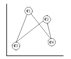
stretched locally ordered som A locally ordered SOM φ stretched out in input space.
stretched globally ordered som A locally and globally ordered SOM φ stretched out in input space.
stretched ordered som SOM arrays stretched out in input space.
To achieve both locally and global order, the neighborhood must be allowed to be wide in the beginning so a rough global ordering can take place among the reference vectors and then by letting it shrink with time, a local structure takes form. So, with topological order is meant a grid structure that is ordered from the beginning (its nodes) and by arranging the associated reference vectors to the nodes so that they also become globally and locally ordered in the grid, then we have the SOM φ .
The formation of the SOM φ can also be thought of as an nonlinear regression of the ordered set of reference vectors into the input space, i.e. the reference vectors in [locally ordered som] forms a elastic grid with the topology of a two-dimensional grid whose nodes have weights as coordinates in the input space and that follows the distribution of the data samples in input space [nonlinear regression process] .
nonlinear regression process initial state
nonlinear regression process middle state
nonlinear regression process final state
nonlinear regression process A nonlinear regression process of the ordered set of reference vectors. nonlinear regression process initial state shows the initial state of the nodes in input space. nonlinear regression process middle state shows how the nodes have moved after a few iteration in their attempts to following the data distribution and at the same arranging the nodes so they have the same ordering as in the grid. nonlinear regression process final state shows the converged SOM φ , i.e. the nodes are placed in areas with high point density and the location of the nodes respective each other corresponds to the initial ordering of the grid nodes.
The overall aim of the algorithm may thus be stated as follows:
Density matching
The SOM φ reflects variations in the statistics of the input distribution: the density of reference vectors of an ordered map will reflect the density of the data samples in input space. In areas with high point density, the reference vectors will be close to each other, and in the empty space between areas with high point density, they will be more sparse.
As a general rule, the SOM φ computed by the SOM algorithm tends to over represent regions of low input density and under representing regions of high input density. One way of improving the density-matching property of the SOM algorithm is to add heuristics to the algorithm, which force the distribution computed by the algorithm to match the input distribution.
The density match is also different for nodes at the border of the grid compared to center nodes at the grid, since the neighborhood to the border nodes are not symmetric. This effect is usually referred to as the border effect and different ways of eliminate these are given in [kohonen01som] . For example, if the batch-map is used, border effects can be eliminated totally if after a couple of batch-map iterations the neighborhood set Ni is replaced by  , i.e. having a couple of simple K-means iterations at the end.
Theoretical aspects of the SOM algorithm
A few words has to be mentioned about the theoretical aspect of the SOM algorithm. How can we be sure that the SOM algorithm converges into a ordered stable state? Frankly, we don't, at least in the multi-dimensional case. It is just a well observed phenomena that the SOM algorithm leads to an organized representation of the input space, even if started from an initial complete disorder. Lets quote Kohonen himself regarding this matter:
"Perhaps the SOM algorithm belongs to the class of "ill posed" problems, but so are many important problems in mathematics. In practice people have applied many methods long before any mathematical theory existed for them and even if none existed at all. Think about walking: theoretically we know that we could not walk at all unless there existed gravity and friction,.... People and animals, however, have always walked without knowing this theory."
It is actually a bit surprisingly that the SOM algorithm has shown such resistant against a complete mathematical study if one consider that the algorithm itself is easy to write down and simulate and that the practical properties of the SOM are clear and easy to observe. And still, no proof for its theoretically properties exists in the general case. These questions are treated by the mathematical expert Marie Cottrell [cottrell98theoretical] in a review paper regarding different proofs of convergence for the SOM algorithm under special circumstances, we quote:
"Even if the properties of the SOM algorithm can be easily reproduced by simulations, and despite all the efforts, the Kohonen algorithm is surprisingly resistant to a complete mathematical study. As far as we know, the only case where a complete analysis has been achieved is the one-dimensional case (the input space has dimension 1) for a linear network (the units are disposed along a one-dimensional array)."
The study of the SOM algorithm in the one dimensional case is nearly complete, all that's left is to find a convenient decreasing rate to ensure the ordering [cottrell98theoretical] . The first proof of both convergence and ordering properties in the one dimensional case was presented by Cottrel and Forth in 1987.
Two obstacles that prevents a thorough study of the convergence of the SOM algorithm in higher dimensions are [kohonen01som] :
How to define ordering in higher dimensions? In the one-dimensional case, ordering of the SOM can easy be defined, but for higher dimensions, no accepted mathematical definition for the ordered states of multi dimensional SOMs seems to exists.
How to define a objective function for the SOM in the high-dimensional case? Only in the special case, when the data set is discrete and the neighborhood kernel is fixed, can a potential function be found in the multi-dimensional case. Ritter proved the convergence in this special case with the use of a gradient-descent method. He then later applied this method to the well-known traveling salesman problem, where the probability density function of input is discrete-valued.
Details and references on actual results in the effort of reaching a solid mathematical theory about the SOM algorithm can be found in [cottrell98theoretical] , as well as in [kohonen01som] .
SOM Toolbox for Matlab
SOM Toolbox(*) [vesanto00som] is an implementation of the SOM and its visualization in MATLAB(*) (MATrix LABoratory). The Toolbox can be used to initialize, train and visualize the SOM. It also provides methods for pre-processing of data, analysis of data and the properties of the SOM. Two SOM algorithms are implemented, the original SOM algorithm and the batch-map. Although we have implemented our own SOM algorithm, the SOM Toolbox provides functions which we have not implemented, such as PCA and Sammon's mapping for analysis of data and some visualization methods.
SOM based applications
The SOM algorithm was developed in the first place for the visualization of nonlinear relations of multidimensional data . However, the properties of the SOM is an interesting tool for two distinct classes of applications:
Simulators used for the purpose of understanding and modeling of computational maps in the brain.
Practical applications such as exploratory data analysis , pattern recognition , speech analysis , robotics , industrial and medical diagnostics , etc.
A complete guide to the extensive SOM literature and an exhaustive listing of detailed application can be found in [kohonen01som] . The first application area of the SOM was speech recognition (speech-to-text transformation). This application was called a 'neural' phonetic typewriter and was developed by Kohonen himself [kohonen88neural] . Another widely known application with Kohonen involved are WEBSOM(*) [kohonen00selforganization] , which is used for content based organization of large document collections and document retrieval. The user interface of the WEBSOM application will be discussed in part III.
Applications of the SOM in recommender systems
This section contains short descriptions of work related in one way or another to ours, in the context of using the SOM in recommender systems.
- CF using SOM and ART2 networks
In [graef01application] they describe two model based approaches to collaborative filtering using SOMs and ART2 networks. They investigate how well the two models performs regarding response time , quality of predictions and adaptively . Their approach to use the SOM algorithm is to cluster users into similar nodes on the grid based on their similarities in rating movies. For this, the EachMovie(*) dataset that contains 2811983 ratings on a scale from 1 to 5 for 1628 movies by 72916 users was used. From this, they randomly selected 2000 users with a minimum of 80 ratings. For their experiments they used a SOM of the size 10x10 nodes. To generate a recommendation for a user, his user-profile is compared to each reference vector and the closest reference vectors is chosen for the recommendation process. This reference vector is then compared with the user and recommendations are made for unrated items in the user profile, i.e. the predicted value is the reference vectors value for the particular movie. To measure the quality of the predictions, 30 ratings was randomly excluded from each user and then one, three, five and 30 recommendations was computed and compared to the excluded ratings for each user. Their test results shows that the SOM made correct recommendations in 45% of the cases for one movie and was correct in 30% of the cases when it had to make 30 recommendations. Compared to their implementation of a collaborative filtering algorithm and the ART2 network, the SOM performed worse. Response time is measured in the cases when the total number of users is 400,1200 and 2000. Not surprisingly, the response time increased with the number of users for the memory based collaborative filtering algorithm, but for both the SOM and the ART2 network, no significant difference can be noted. This has to do with the fact, that the SOM only has to do 100 comparisons, no matter how many users there are, as in contrast to the memory based collaborative filtering algorithm that has to make as many comparisons as there are users. Adaptively means the SOMs ability to adapt to new users without having to re-learn the whole SOM. The SOM clearly outperformed the ART2 network on this, no distinct difference could be detected between the number of correct recommendations made by an updated SOM and a re-learned SOM.
- Hybrid recommender system combining CF with SOM
A hybrid recommender system that combines CF with the SOM is presented in [lee02hybrid] . Their approach is to use the SOM algorithm as a cluster algorithm in which the clusters are formed according to the users demographic data (sex and age) and preferences for different movie genres as action, drama, comedy, fiction and thriller. the idea is then to apply collaborative filtering on the cluster to which the active user belongs. They claim that their solution is comparable with the collaborative filtering algorithm introduced by GroupLens [resnick94grouplens] based on the computed mean absolute error. However the data set they uses consists of only 174 users and 53 movies and no characteristics is presented for this unknown data set. Also, coverage is not reported at all.
- CBR-CF with SOM as a clustering algorithm
In [roh03cbr] a cluster-indexing case based reasoning (CBR) model for collaborative filtering recommendations are described. Their approach is to use the SOM algorithm as a clustering algorithm and then use the reference vectors as indexes for where similar users (or cases in CBR terminology) can be found in the case-base reasoning process. Clusters are formed according to the users ratings on movies, the well-known MovieLens data set is used, however, they only uses a fraction of the data set, a dense rating matrix with 251 users and 33 movies are used for evaluation. PCA has been used for a pre-step analyzing of the data set and from their experiments, the size of the grid is set to four nodes (clusters). Prediction for the active user is done by finding the active users closest reference vector and then applying collaborative filtering with the users indexed by the same reference vector. Their studies show comparable results compared to collaborative filtering techniques based on the reported normalized mean absolute error.
- Music artist reviews SOM
A content-based approach is taken in [vembu04selforganizing] , very much similar to earlier studies done by the authors of this thesis [gabrielsson04movsom] . Their idea is to use music artist reviews taken from Amazon web site and extract words from the reviews to build artist-profiles. The usual techniques found in text-retrieval is used to form these artist-profiles; vector space model and tf-idf weighting schema. They also hand-picked 324 words that they thought to be of extra importance that was given extra weight in the artist-profiles. The dimension of the artist-profile was reduced to 3313 from original 36708 by excluding words that was present in less than 5% and more than 90% of the artist reviews.
The SOM algorithm was then used to cluster artist-profiles represented as bag-of-words. They implemented a SOM of size 7x7 nodes using the SOM Toolbox for 398 artists. Evaluation was made by comparing their SOM against a web-based music recommendation engine. Each BMN contains artists similar to each other based on artist reviews and the web-based engine recommends artists similar to a specific artist, but from a much larger data set and with a completely different approach. The top 10 list generated by the web-engine for a specific artist was compared to the BMN for the same artist. Observations was made that if they included the artist top 3 or 5 BMN, the overlap between the top 10 list and the artists neighbourhood increased. Which of course is by the virtue of the map's self-organizing property, neighbouring nodes represents similar data.