Chapter 3 - Artificial neural networks
Artificial neural network is a discipline that draws its inspiration from biological neural networks in the human brain. Artifical neural networks resembles the brain in two respects: the network acquires knowledge from its environment using a learning process (algorithm) and stores the learned information in interneuron connection strengths called synaptic weights . At the cellular level, the human brain consists primarily of nerve cells called neurons . Neurons are parallel working units connected to each other in a network style. The human brain contains approximately 1011 neurons. Each of these neurons is connected to around 103 to 104 other neurons, and therefore the human brain is estimated to have 1014 to 1015 connections. The neuron is the basic building block of the nervous system and most neurons are to be found in the brain.
The brain
The brain can be seen as a highly complex , nonlinear , and parallel information-processing system . It has the capability of organizing neurons so as to perform certain computations (e.g. pattern recognition, perception, and motor control) many times faster than the fastest digital computer. The brain is almost completely enveloped by the cerebral cortex. Although it is only about 2-3 mm thick, its surface area, when spread out, is about 2000 cm2 (roughly three times this paper). Typically, neurons are five to six orders of magnitude slower than silicon logic gates; events in a silicon chip happen in the nanosecond ( 10-9 s) range, whereas neural events happen in the millisecond ( 10-3 s) range. However, the brain makes up for the relatively slow rate of operation of a neuron by letting its huge number of neurons operate in parallel. The net result is that the brain is an enormously efficient structure [haykin94neuralnetworks] .
The long course of evolution has also given the human brain many other characteristics that are desirable in an artifical neural network. Some of these include:
- Robustness and fault tolerance
Nerve cells can die without any significant loss of performance by the brain.
- Adaptivity and learning
The brain is trained - not programmed - and adapts therefore easily to new environments.
- Fuzziness
Information can be inconsistent and noisy.
- Massive parallelism
At birth, the distinct areas of the brain are all at place and within each brain area are millions of neurons that are connected to each other by synapses . These synapses and the pathways they form make up the neural network in the brain. After birth, the brain development continues and consists of wiring and rewiring the connections (synapses) between neurons. New synapses are created and old ones disappears, all depending on what kind of experience the brain is exposed to. The most dramatically development of the brain takes place in the first two years from birth but it continues well beyond that stage. During this early stage of development, about one million synapses are formed per second.
The biological neuron
Neurons can be of many types and shapes, but ultimately they function in a similar way and are connected to each other in a rather complex network stylish way via strands of fibre called axons . A neurons axon acts as a transmission line and are connected to another neuron via that neurons dendrites , which are fibres that emanate from the cell body ( soma ) of the neuron. The junction that allows transmission between the axons and the dendrites are the synapse. Synapses are elementary structural and functional units that creates the signal connection between two or more neurons; sometimes meaning the connection as whole. [neuron synapse] (*)
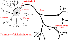
biological neuron Schematic view of a biological neuron.
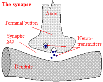
synapse The Synapse.
neuron synapse Within the brain the biological neurons are connected by way of synapses.
The most common kind of synapse is a chemical synapse: when a neuron is stimulated, it transmit that nerve pulse to another neuron through the axons and causes the release of neurotransmitters that travel through the synapse to the other neuron. That is, a presynaptic process liberates a transmitter substance that diffuses across the synaptic junction between neurons and then acts on a postsynaptic process. Thus a synapse converts a presynaptic electrical signal into a chemical signal and then back into a postsynaptic electrical signal. In traditional descriptions of neural organization, it is assumed that a synapse is a simple connection that can impose excitation (positively) or inhibition (negatively) on the receptive neuron.
A developing neuron is synonymous with a plastic or adaptive brain. Plasticity permits the developing nervous system to adapt to its surrounding environment, i.e. the creation of new synaptic connections between neurons and the modification of existing synapses. It is this type of adaptation that forms the basis for learning. Since plasticity appears to be essential to the functioning of neurons as information processing units in the human brain, the same goes for neural networks made up of artificial neurons. A phrase that sometimes appears in the context of artifical neural networks is the stability-plasticity dilemma , which refers to the dilemma of a system having to be adaptive enough to allow for learning of new knowledge (plasticity) while not forgetting previous learned knowledge (stability).
The artificial neuron
Artificial neurons are information-processing units that are only approximations (usually very crude ones) of the biological neuron [artificial neuron] . Three basic elements of the artificial neuron can be identified [haykin94neuralnetworks] :
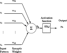
artificial neuron Artificial neuron
A set of synapses or connection links , each of which is characterized by a weight or strength of its own. Specifically, a component xi at the input of synapse i connected to a neuron k is multiplied by the synaptic weight wik . Note that the first subscript of the weight refers to the input end of the synapse and the second to the neuron in question. The weight wik is positive if the associated synapse is excitatory; it is negative if the synapse is inhibitory.
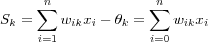
An summation function for summing the input signals, weighted by the respective synapses of the neuron and producing a linear output Sk . Sometimes referred to as a linear combiner.
An activation function for limiting the amplitude of the output of a neuron. In general, activation functions are monotonically increasing functions, where, (excluding the linear function) (
 or f(8) = -1 ) and f(8) = 1 , i.e. the output of a neuron can be written as the closed unit interval [0, 1] or alternatively [-1, 1] .
The model of a neuron also includes an fixed input x0 = 1 and a weight  called the threshold. Mathematically, we can describe the artificial neuron as follows:

where  are the input signals;
  are the synaptic weights of neuron k ; S is the sum of the input signals and the threshold; f(Sk) is the activation function and yk is the output signal of neuron k .
The computational process can be described as follows: an artificial neuron receives its inputs  from some external source (the real world), computes a weighted sum S (usually) of the input signals (including the threshold) using the summation function. This sum S is then used as input for the activation function f(S) that generates the final output y .
Different types of activation functions can be used and three of them are described in [activation functions] . The most commonly used is nonlinear sigmoid activation functions such as the logistic function . A logistic function assumes a continuous range of values form 0 and 1 in contrary to the discrete threshold function. A binary threshold function was used in the first model of an artificial neuron back in 1943, the so-called McCulloch-Pitts model . Threshold functions goes by many names, e.g. step-function , heavyside function , hard-limiter etc. Common for all is that they produce one of two scalar output values (usually 1 and -1 or 0 and 1) depending on the value of the threshold. Another type of activation function is the linear function or some times called the identity function since the activation is just the input. In general if the task is to approximate some function then the output nodes are linear and if the task is classification then sigmoidal output nodes are used.
Mathematically and graphically, we can describe the functions as in [activation functions] .
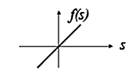
linear activation function Linear function
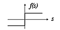
threshold activation function Threshold function
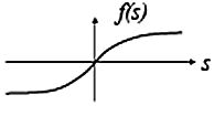
sigmoid activation function Sigmoid function
activation functions linear activation function The linear function  produces a linearly modulated output, where α is a constant (if α is 1 it becomes the identy function). threshold activation function The threshold function f(S) in this cases uses a threshold of zero causing the output to be either 1 or -1, i.e. f(S) = 1 if
  and -1 if
  . sigmoid activation function In the sigmoid function
  that is shown (the logistic function) λ controls the steepness of the function, and is usually equal to -1.
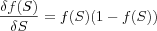
A nice property of the sigmoid function is that its derivative [sigmoid derivative] is easy to calculate, which is an important feature in network theory.
If every aspect of a biological neuron was to be considered in a computer simulation, then one would need more than all the computing resources that are available to theorist now days [kohonen01som] . Therefore, artificial neurons and hence, artifical neural networks are only approximations to parts of the real brain, and the extent to which a artifical neural network approximate a particular part of the brain usually varies. This means, that if the goal is to understand the principles on which the human brain works, then the biological plausibility of the artifical neural network is of primary concern, otherwise, the artifical neural network models can been seen as practical inventions for new components and techniques inspired by the brain.
Formal definition of artificial neural networks
From a practical point of view, an artifical neural network is a parallel computational systems , inspired by the structure , processing methods and learning ability of the human brain, consisting of many simple processing elements (artificial neurons) connected together in a specific way (network style) in order to perform a particular task.
One of the most powerful features of artifical neural networks are their ability to learn and generalize from a set of training data . Training data is used only for training the network to perform a certain task. In order to test how good the network is on performing the particular task it has been trained for, a special data set called test data is used that contains examples that was not included in the training set. Learning means that the network adapt the strengths/weights of the connections between neurons until enough knowledge about the training data is stored in the network so it can perform the task it been trained for. Generalization means that the network after training can recognize inputs correctly that was not part of the training dataset, hence the importantly of using test data that has not been included in the training data. Note that knowledge is stored in the weights not in the neurons, i.e. the final configuration of the weights represent the networks knowledge. Four basic rules when it comes to knowledge representation in a neural network are given in [haykin94neuralnetworks] :
Similar inputs from similar classes of input should usually produce similar representations inside the network.
Data categorized as belonging to separate classes should give widely different representations in the network.
If a particular feature is important, then there should be a large number of neurons involved in the representation of that data in the network.
Prior information and invariance's should be built into the design of a neural network, thereby simplifying the network design by not having to learn them.
From the above discussion, we can adapt Haykins definition of a neural network [haykin94neuralnetworks] :
"A neural network is a massively parallel distributed processor that has a natural propensity for storing experiential knowledge and making it available for use. It resembles the brain in two respects:
Knowledge is acquired by the network through a learning process.
Interneuron connection strengths known as synaptic weights are used to store the knowledge."
The procedure used to perform the learning process is called a learning algorithm , the function of which is to modify the synaptic weights of the network. The modification of synaptic weights provides the traditional method for the design of neural networks, however, it is also possible for a neural network to modify its own topology, which is motivated by the fact that neurons in the brain can die and that new synaptic connections can grow.
Artifical neural network structures and learning algorithms
[artificial neuron structure] provides a functional description of the various elements that constitute the model of an artificial neuron. A more simpler way of representing the structure of an artificial neuron and particular artificial neural networks is with the so-called so-called architectural graph [Figure 48] which describes the layout of an artifical neural network. Haykin [haykin94neuralnetworks] also represents neural networks in terms of signal-flow graphs in which artificial neurons are nodes and directed links are connections between nodes. In the terms of a signal-flow graph, the architectural graph is to be considered as a partially complete signal-flow graph.
artificial neuron structure The structure of a artificial neuron.
Two main structures of artifical neural networks, based on the arrangement of nodes and the connection patterns of the layers, are feedforward networks and recurrent networks. A layered neural network is a network of neurons organized in the form of layers. In the simplest form it consists of one input layer of source nodes and one output layer consisting of one or more neurons. However, multilayered networks are by far the most common architecture of any neural network, in particular the popular multilayer perceptrons feedforward network. The difference is the presence of one or more hidden layers of neurons. The function of the hidden neurons is to intervene between the external input and the network output, typically, the neurons in each layer of the network have as their inputs the output signals of the preceding layer only. By adding one or more hidden layers, the network is capable of modeling more complex relationships between the input variables and the output variables.
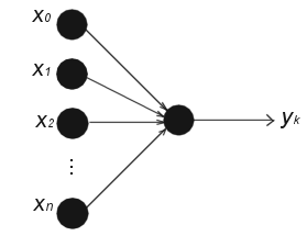
Feedforward networks
The name "feedforward" came from that neuron interconnections are acyclic, i.e. input nodes are connected to output nodes, but not vice versa. [artificial neuron structure] actually shows an Single-Layer Feedforward network consisting of only one neuron in the output layer. Another class of feedforward networks are multilayer Feedforward networks , as shown in [fully connected feedforward network] . A feedforward network can be fully or partially connected in the sense that every node in each layer is either connected or not connected to every node in the adjacent forward layer. Another type of feedforward network is called a lattice network in which the output neurons are arranged in rows and columns. Usually the lattice consists of one or two-dimensional array (although higher dimensions are possible) of neurons with a corresponding set of source nodes. Each source node is connected to every neuron in the lattice [fully connected feedforward lattice network] . The most known example of this kind of network is Kohonen's SOM.
Recurrent networks
Recurrent network has input nodes, hidden neurons, output neurons, just as feedforward networks, what distinguish themselves from feedforward networks is that they have at least one feedback loop, i.e. when a neurons output is fed back into the network as input. A special type of feedback loop are called self-feedback loops, which refers to a situation in which the output of a neuron is fed back to its own input. Another type of feedback loop introduces a new type of nodes called context nodes [fully connected recurrent network] . These nodes receive connections from the hidden neurons or the output layers of the network and have output connections that travel back to the hidden neurons. Context nodes are required when learning patterns over time (i.e. when the past value of the network influences the present processing). Recurrent networks can therefore be seen as an attempt of incorporate time and memory into a neural network Two examples of recurrent networks that are simple extensions of feedforward networks are Jordan network (feedback from output layer to input layer) and Elman network (feedback from hidden layer to input layer). Also, a widely known recurrent network is the Hopfield network in which all the connections are symmetric.
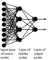
fully connected feedforward network A (fully connected) multilayer feedforward network
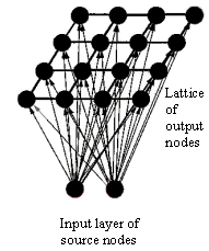
fully connected feedforward lattice network A fully connected feedforward 2-dimensional lattice network
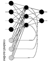
fully connected recurrent network A fully connected recurrent network with three context nodes
networks Neural networks
The structure of an artifical neural network is closely related with the learning algorithm used to train the network, different network architectures require appropriate learning algorithms.
Learning Rules
A learning algorithm refers to a procedure in which learning rules are used for adjusting the weights, which formally can be defined in the context of neural networks as follows [haykin94neuralnetworks] :
"Learning is a process by which the free parameters (the weights) of a neural network are adapted through a continuing process of stimulation by the environment in which the network is embedded. The type of learning is determined by the manner in which the parameter changes take place.
Which implies the following sequence of events:
The neural network is stimulated by an environment.
The neural network undergoes changes as a result of this stimulation.
The neural network responds in a new way to the environment, because of the changes that have occurred in its internal structure."
Mathematically, this can be describes as follows. Let wik(t) denote the value of the synaptic weight wik at time t between two neurons i and k or a input node i and a neuron k . At time t an adjustment  is applied to the synaptic weight wik(t) , yielding the updated value:

where wik(t) and wik(t+1) is the old and new values of the synaptic weight wik and  is the adjustment applied to the old value of wik as a result of the stimulation from some environment.
The reason why time is involved in the equation is that the network gradually adapts the synaptic strengths, so t can be regarded as the number of times the neuron has been updated, or how many training examples that has been run trough.
There is no unique learning algorithm for the design of neural networks, different learning algorithms has advantages of their own. In general, learning algorithms differ from each other in the way in which the adjustment  to the synaptic weight wik is formulated.
Four basic types of learning rules are [haykin94neuralnetworks] : error-correction learning , Hebbian learning , competitive learning and Boltzmann learning . Error-correction learning is rooted in optimization theory whereas Hebbian and competitive learning are inspired by neurological considerations. Boltzmann learning is different altogether in that it is based on ideas borrowed from thermodynamics and information theory. A brief explanation of error correction learning, Hebbian learning and competitive learning will be described below. Competitive learning will also be described in more detail in the next chapter on SOMs.
Error-correction learning
Typically, the actual output yk(t) produced by some vector x(t) applied to the input of the network at time t in which neuron k is embedded differs from the desired output dk(t) . Let the difference between the desired and actual output define an error signal 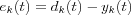 .
.
The error signal ek(t) is then used to adjust the values of the synaptic weights so that the output signal approaches the desired response dk(t) in a step-by-step manner.
The simplest form of error-correction rule is the perceptron convergence procedure , invented by Rosenblatt in the 50s and published 1960. This rule is nonlinear, adjusting the weights makes use of the "quantize error" ek , defined to be the difference between the desired output dk and the output of the quantiziser yk , e.g. a binary threshold activation function [widrow90perceptrons] . The weights are updated using [weight update] with:
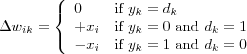
That is, if ek = 0 , no adjusting of the weights takes place. Otherwise, updating the weights is done by adding the input vector x to the weight vector w if the error is positive, or by subtracting the input vector x from the weight vector w if the error is negative. The input xi is also multiplied with a positive learning-rate parameter η . For stability, the learning rate should be decreased to zero as iterations progress and this affects the plasticity.
Another type of error correction rule is based on the gradient descent method . The purpose of the gradient descent method is to minimize a cost function based on the error signal ek(t) , such that the actual response of each output neuron in the network approaches the target response for that neuron. Once a cost function has been chosen, this becomes an optimization problem(*) to which the theory of optimization can be applied.
A criterion commonly used for the cost function is the instantaneous value of the mean-square-error criterion
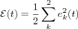
where summation is over all neurons in the output layer.
The network is then optimized by minimizing the error function  with respect to the synaptic weights of the network. The weights are updated using [weight update] with:
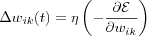
The learning-rate parameter η is a positive constant which determines the amount of correction. Thus,  is the adjustment (correction) made to weight wik(t) at time t .
The derivation of

using the notation from [artificial neuron structure] , i.e. the derivative of the cost function Ε with respect to the weights is calculated using the chain rule which gives us the following partial derivatives:
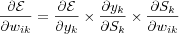
which are equal to:
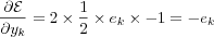
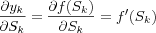
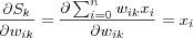
Hence
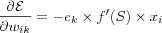
Which, in general form is:

where wik(t) is the i-th element of the weight vector wk(t) of the output neuron k and xi is the corresponding i -th component of the input vector x(t) .  is the derivative of the activation function.
The first ones to published such a rule was Windrow and Hoff, who in 1960 published the least mean square algorithm or Windrow-Hoffs delta rule as it also is referred to. This rule is linear, adjusting the weights makes use of the "linear error" ek , defined to be the difference between the desired output dk and the output of the linear combiner [widrow90perceptrons] , hence yk = Sk , if we use the notation from [artificial neuron structure] . Which gives,  , and since
  , its derivative is equal to 1. Using [general weight adjustment] , we get that:

The weights are then updated using [weight update] .
This learning rule is also local since it uses information directly available to neuron k through its synaptic connections. The learning rate parameter η is crucial to the performance of error-correction learning in practice as it determines stability, convergence speed and the final accuracy.
A generalization of this rule is called the generalized delta learning rule and assumes continuous activation functions which are at least once differentiable, hence the popular choice of the logistic function as the activation function, since it is both continuous and has an easy calculated derivative. We will not go in to detail here, but this generalization makes it possible to train multilayer networks with sigmoidian activation functions in the hidden layer. The rule is nonlinear and adjusting the weights makes use of the "sigmoidian error" ek , defined to be the difference between the desired output dk and the output of the sigmoidian yk (e.g. the logistic function).
The most popular learning algorithm that implements this is the backpropagation algorithm. This algorithm consists of two phases:
Feedforward pass , in which the output error is calculated.
Backward propagation , in which the error signal is propagated back from the output layer toward the input layer and on its way to the input layer, the weights are adjusted as functions of the backpropagated error, hence the name of the algorithm.
The principle is the same as for the delta rule, we are only applying it to more nodes in several layers and making the chain in the chain rule a bit longer.
To illustrate the gradient decent method, we can plot the error function against the weights. This plot illustrates a multi-dimensional weight space, usually called the error-surface . In the linear case, e.g. the least mean square algorithm, the error function becomes quadratic in its parameters and a global minimum solution can easily be found. A plot for the error surface for one weight in the linear case is shown in [linear error surface] .
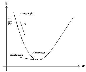
linear error surface The error surface in the linear case for one weight. The gradient of E in weight space are calculated and the weight are moved along the negative gradient.
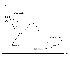
nonlinear error surface The error surface in the nonlinear case for one weight. The gradient of E in weight space are calculated and the weight are moved along the negative gradient.
error surface Error surfaces
However, in most cases the output of an artifical neural network is a nonlinear function of its parameters because of the choice of the activation function, e.g. the sigmoid functions, which is the case in the general delta rule. As a result, it is no longer straightforward to derive at a solution for the weights that is guaranteed to be globally optimal. In the case of the back-propagation algorithm, one way to avoid this is to add a momentum term into the equation. This is easier pictured if we think of the solution as a ball on the error surface, bouncing back and fourth, and whenever it got trapped in a local minimum on the error surface, that extra momentum term will enforce that ball to bounce out of that minima and keep it bouncing until it got trapped in a global minima. At least, that's the idea. A plot of a nonlinear error surface is shown in [nonlinear error surface] for one weight.
In the case of SOMs, discussed in detail in the next chapter, it has been proven that it is impossible to associate a global decreasing cost function to the SOM in the general case [erwin92ordering] .
Hebbian Learning
Within the field of artificial neural networks, Hebbian learning is an unsupervised training algorithm in which the synaptic weight wik (strength) from neuron i to neuron k is increased if both neuron i and neuron k are active at the same time. A natural extension of this is to decrease the synaptic strength when the source neuron i and output neuron k are not active at the same time. Hence, the adjustment applied at time t to the synaptic weight wik with presynaptic and postsynaptic activities denoted by xi and yk can be expressed in mathematical terms as:

where F is a function of both the postsynaptic and presynaptic activities.
As a special case we may use the activity product rule:
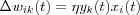
where η is the learning rate parameter.
Hence, Hebbian learning can then be expressed as:

Of course, from this representation we see that the repeated application of the input signal xi leads to an exponential growth that finally drives the synaptic weight wik into saturation. One way to avoid this is to impose some sort of limit on the growth of synaptic weights. One method for doing this is to introduce a forgetting factor into the formula as follows:

where α is a new positive constant and wik(t) is the synaptic weight at time t .
Equivalently, we can write the above expression as the generalized activity product rule :
![\Delta w_{ik}(t) = \alpha y_k(t)[c x_i(t) - w_{ik}(t)]](image/equation58.png)
where c =  . If the weight wik(t) increases to the point where
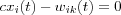
a balance point is reached and the weight update stops.
Competitive learning
Competitive learning is a process in which the output neurons of the network compete among themselves to be activated with the result that only one output neuron, is on at any time. There are three basic elements to a competitive learning rule [haykin94neuralnetworks] :
A set of similar neurons except for some randomly distributed synaptic weights. Therefore the neurons respond differently to input signals.
A limit imposed on the strength of each neuron.
A competing mechanism for the neurons.
The output neurons that wins the competition are called winner-takes-all neurons and as a result of the competition, they become specialized to respond to specific features in the input data. In the simplest form of competitive learning, the neural network has a single layer of output neurons, each of which is fully connected to the input nodes [competitive neural networks] .
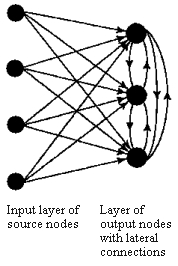
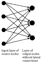
competitive neural networks Two simple forms of a competitive neural network. Feedforward connections from source nodes to the neurons are excitatory and the connections among the neurons are inhibitory.
The network may include lateral connections among the neurons, as shown in [competitive neural networks] , and thereby perform lateral inhibition, with each neuron tending to inhibit the neuron to which it is laterally connected. A neuron k is the winning neuron if its net internal activity level Sk for a given input vector x is the largest one among all neurons in the network, where Sk is the combination of all the forward and feedback inputs for neuron k . The output signal yk of winning neuron k is set to one and all the others to zero. Each neuron is allowed a fixed amount of synaptic weight (typically, all synaptic weights are positive), which is distributed among its input nodes; that is, we have  for all k and where wik denotes the synaptic weight between input node i and neuron k . A neuron learns by shifting synaptic weights from its inactive input nodes to the active ones, no learning takes place if the neuron don't respond to a particular input vector x . The change
  applied to synaptic weight wik is defined by the standard competitive learning rule:
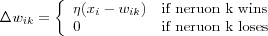
where η is the learning parameter. The effect of this rule is that the synaptic weight vector wk of the winning neuron k is moved toward the input vector x .
Learning paradigms
Another factor to be considered is the manner in which a neural network relates to its environment during learning, i.e. what kind of information is available to the network. In this context, a learning paradigm refers to an model of the environment in which the neural network operates. There are three main learning paradigms: supervised , unsupervised and reinforcement learning . Kohonen [kohonen01som] explains the difference in the three learning paradigms as follows.
- Supervised learning
Learning with a teacher, i.e. a learning scheme in which the average expected difference between wanted output for training samples and the true output is decreased, using e.g. the backpropagation algorithm.
- Unsupervised learning
Learning without a priori knowledge about the classification of samples, i.e. learning without a teacher. Often the same as formation of clusters, after which the clusters can be labeled, e.g. Kohonen's SOM algorithm.
- Reinforcement learning
Learning mode in which adaptive changes of the parameters due to reward or punishment depend on the final outcome of a whole sequence of behavior. The results of learning are evaluated by some performance index.
Learning protocols
The ways in which the input vectors are presented to the networks determine the learning protocol in which the network learns its environment by adjusting its parameters. Two main principles are the following ones:
- Incremental Learning
Weights are updated after each presentation of a training vector x . Also known as pattern learning or stochastic learning if the training vectors are choose randomly.
- Batch Learning
Weights are updated after all training vectors have been presented once for the network, i.e. the changes of the weights are accumulated until all vectors in the training set has been presented. Also known as epoch learning.
A brief history of artificial neural networks
We will round off this short introduction to artificial neural networks with a brief look at some important milestones within the research field of neural networks(*) .
One early reference concerning the theory about neural networks can be made to Alexander Bain [wilkes97bain] . In his book "Mind and Body: Theories of their relation" from 1873, he relates the process of associative memory to the distribution of activity in neural grouping or neural networks in modern terms. He found out that individual nerve cells carrying excitatory links to selected other cells within a grouping, that each nerve cell is summating the degree of stimulation it receives from other parts of the network, and that the same network can generate different output depending on its internal connections. And what even more interesting is that his rule for associations (groupings) precedes that of a later ones, better known as Hebb's hypothesis from 1949. With Bains own words as reprinted in [wilkes97bain] :
"when two impressions concur, or closely succeed one another, the nerve currents find some bridge or place of continuity, better or worse, according to the abundance of nerve matter available for the transition. In the cells or corpuscles where the currents meet and join, there is, in consequence of the meeting, a strengthened connection or diminished obstruction -- a preference track for that line over lines where no continuity has been established."
Bain emerges as the first theorist that goes beyond generalized statements towards providing detailed examples and network drawings. Unfortunatly, Bain himself came to doubt about his work and not even one of his own students, David Ferrier who published the classical work "The Functions of the Brain" in 1876 mention the details of Bains work. Therefore, much of what Bain discovered is now credited by other researchers.
However, the modern era of neural networks is said to have began with the pioneering work of McCulloch and Pitts in the 40s. Warren McCulloch (a psychiatrist and neuroanatomist) and Walter Pitts (a mathematician and logician) published a paper 1943 entitled "A logical calculus of the ideas immanent in nervous activity" in the Bulletin of Mathematical Biophysics. In this paper, they proposed a mathematical model of a biological neuron based on the all-or-nothing theory of biological neurons, i.e, the output from a neuron is constant; either it is maximal or its nothing. What they proposed was a binary threshold unit as a computational model for an artificial neuron which corresponded to their view of the nervous system as a network of finite interconnection of logical devices. The McCulloch-Pitts neuron works on binary signals and in discrete time; they receive one or more input signals and produce an output signal in a similar way as described earlier in figure 2. The activation function they used was a binary threshold function or step function, with a threshold at 0. The central conclusion of their paper was that any finite logical expression can be realized by a network built of McCulloch-Pitts neurons. This conclusion was important in the sense that it showed that networks of rather simple elements connected together can be computationally very powerful. However, in their model, the weights are constant, there is no learning. The McCulloch-Pitts paper had an great influential, and it was not long before the next generation of researchers added learning and adaptation.
Donald O. Hebb, a Canadian neurophysiologist, presented in his book "The Organization of Behaviour" , from 1949 a theory of behaviour based on the physiology of the nervous system. The most important concept to emerge from this work was his formal statement (known as Hebb's postulate) of how learning could occur. Learning was based on the modification of synaptic connections between neurons. Specially, as restated in [haykin94neuralnetworks] ,
"When an axon of cell A is near enough to excite a cell B and repeatedly or persistently takes part in firing it, some growth process or metabolic change takes place in one or both cells such that A's efficiency, as one of the cells firing B, is increased."
The principle underlying this statement have become known as Hebbian learning.
Hebb was proposing not only that, when two neurons where active together the connection between the neurons is strengthened, but also that this activity is one of the fundamental operations necessary for learning and memory . This meant that the McCulloch-Pitts neuron had to be altered to at least allow for this new biological proposal.
One of the first to exploit this idea, to make a learning rule for artificial neurons, was Frank Rosenblatt in the late 50s. He used the McCulloch-Pitts neuron and the findings of Hebb in the developing of the perceptron . The perceptron was originally designed as a linear pattern(*) classifier, i.e, used for the classification of a special type of patterns, which are linearly separable . This means that the input vectors can be seen as points in a N -dimensional input space and what the perceptron does is to put a discriminant in this space. This discriminant defines a hyperplane in the N -dimensional space.
In two dimension this discriminant is a line and can be found where the linear output Sk equals zero:

therefore
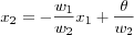
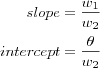
[and classifier] graphs this linear relation, which comprises a separating line having slope and intercept given by:
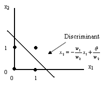
and classifier A 2-dimensional input space. Four points  ,
,  ,
,  and
and  in a two dimensional input space are spanned by x1 and x2 . Training of a perceptron with two inputs x1 and x2 would then be to adjust the weights w1 and w2 such that the weights (and the threshold
  with x0 = 1 ) defines the slope and position of a line that separates the points into two classes. In this case class one consists of the points
  ,
,  ,
,  and class two of the single point
  .In this particular case, the perceptron has been trained to implement the boolean function AND, i.e. when its fed with the points from class one, it will output 0 (false) and the point from class two will yield a 1 (true). It acts just as a logic gate as in McCulloch and Pitts case. The difference is that the perceptron is able of finding suitable weights automatically.
Rosenblatt's learning algorithm, referred (as previously described) to as the perceptron convergence procedure , was used to train the perceptron. Although the core idea of the perceptron was the incorporation of learning into the McCulloch-Pitts neuron, the thing that really caused a lot of enthusiasm in the world of computer science was that Rosenblatt presented this learning algorithm together with a theorem, called the perceptron convergence theorem . This theorem says that this learning algorithm will converge to an optimal discriminant in a number of finite steps, if such a discriminant exists . This theorem created a big hype regarding perceptrons and caused a lot of activity in the 50s and the 60s, people thought that now we can compute anything, solve any problem, we don't have to program anymore and so on. Unfortunately, a lot of people most have missed this last point, because its not always true, which will soon be explained why.
About the same time as Rosenblatt, Bernard Widrow and Marcian 'Ted' Hoff of Stanford developed the Adaline (ADAptive LInear NEuron) which was very similar to the perceptron. The adaline is an adaptive threshold logic element with a hardlimiter activation function outputting +-1 . The principal difference between the perceptron and the adaline lies in the training procedure, adaline uses the least mean square algorithm, as explained earlier, to train the adaline [widrow90perceptrons] .
Unfortunately, both Rosenblatt's and Widrow's networks suffered from the same inherent limitations, which were publicized in the influential book "Perceptrons: An Introduction to Computational Geometry" in 1969 by Minsky and Papert. This book contained a detailed analysis of the capabilities and limitations of perceptrons. In their book, Minsky and Papert used the XOR-problem as an example for the demonstration that the perceptron can only do linearly separable problem. Of course, this was nothing new among those who did research on perceptrons and its variants, Rosenblatt himself had done some research regarding this [carpenter89neural] . The XOR problem can be considered as a classification problem for the perceptron to solve. That is, the perceptron can be constructed as a XOR logic function that has two inputs  and one output y which should equal 1 if the input is
  or
or  and a 0 if the input is
  or
or  , see the truth table for the exclusive-or function in [xor] . This input space can be plotted as in [xor classifier] and the aim of the perceptron is to find a discriminant that separates this points.
TROUBLESOME MINIPAGE FIGURE
As can be seen from [xor classifier] , no single line can separate the points, e.g. the problem is linearly inseparable. A perceptron cannot solve any problem that is linearly inseparable. The solution to the XOR problem in this case is to use more than one perceptron, e.g. multilayer perceptrons . In the first layer, two perceptrons are set up to identify small, linearly separable sections of the inputs, e.g. one perceptron implements the OR function and the other implements the AND function and then combining their outputs into another perceptron in the output layer, which produce a final indication of which class the input belongs to. Of course this solution to the XOR problem, that it is possible to construct a network with layers of perceptrons with predefined weights, was also widely known. But what Minsky and Papert's stated in their book was that it is not possible to find a learning algorithm that can find the correct weights automatically . This problem is also known as the credit assignment problem , since it means that the network is unable to determine which of the input weights should be increased and which should not, i.e. the problem of assigning credit to the perceptrons in the network so they can produce a better solution next time.
This hasty conclusion made by Minsky and Papert's had some devastated effects on the research community, lot of people that financed this kind of research read this book, and almost over one night, all funding into this field was stopped. This, combined with the fact that there were no powerful computers at the time to run experiments on, caused many researchers to leave the field. For example, a research team [haykin94neuralnetworks] involved in the developing of a nonlinear learning filter, spent six years building the filter with analog devices.
The years that followed is sometimes referred to as the "ice age" by researchers in the neural network community, because almost no one looked into the fields of neural networks except for researchers in psychology and neuroscience, but from a physics and engineering perspective, the field was almost completely dead [haykin94neuralnetworks] . This period of time lasted between 1969 to mid 80s. Despite this, some important activities and results was made during this period, where some notable ones are the work by James Anderson and Teuvo Kohonen on associative memories in 1972 and the pioneering work on competitive learning and self-organizing maps by von der Malsburg [vondermalsburg73selforganization] , Stephen Grossberg [grossberg76adaptive] and also Kunihiko Fukushima, who explored related ideas with his biologically inspired Cognitron [fukushima75cognitron] and Neocognitron [fukushima80neocognitron] models. It was also during this time period that Kohonen began his work on SOMs that he later published in 1982 [kohonen82selforganizing] .
The interest in neural networks re-emerged after two important theoretical results were attained in the early eighties. In 1982, the American scientist John Hopfield used the idea of an energy function to formulate a new way of understanding the computation performed by recurrent networks with symmetric synaptic connections. This had the positive effect that physics became interested in the field. The second was the solution to the credit-assignment problem by the rediscovery of the backpropagation algorithm in 1986. By replacing the discontinuous threshold function used by the perceptron with a continuous smooth "sigmoid function" one could use the generalized delta rule, as explained earlier, for the minimization of the output error, i.e. it was now possible to find out how much credit should be assign to the perceptrons so their weights could be updated.
This algorithm was in fact described as early as 1974 by Paul Werbos in his Ph.D. thesis "Beyond regression: new tools for prediction and analysis in the behavioral sciences" at Harvard University. Werbos's work should unfortunately remain almost unknown in the scientific community until 1986, when Rumelhart, Hinton, and Williams rediscovered the technique and, within a clear framework, described their work in the article "Learning Internal Representations by error propagation" , published in the two-volumed book "Parallel Distributed Processing: Explorations in the Microstructures of cognition" by Rumelhart and McClelland, in that same year. This contributed to making the method widley known and this book has since then been a major influence in the use of back-propagation learning.
In the last twenty years, thousands of papers have been written, and neural networks have found many applications such as character recognition, image recognition, credit evaluation, fraud detection, insurance, and stock forecasting. The field is showing new theoretical results and practical applications. The use of neural networks as a tool to be used in appropriated situations and the fact that we know very little about how the brain works makes the future of neural networks to look very promising.